

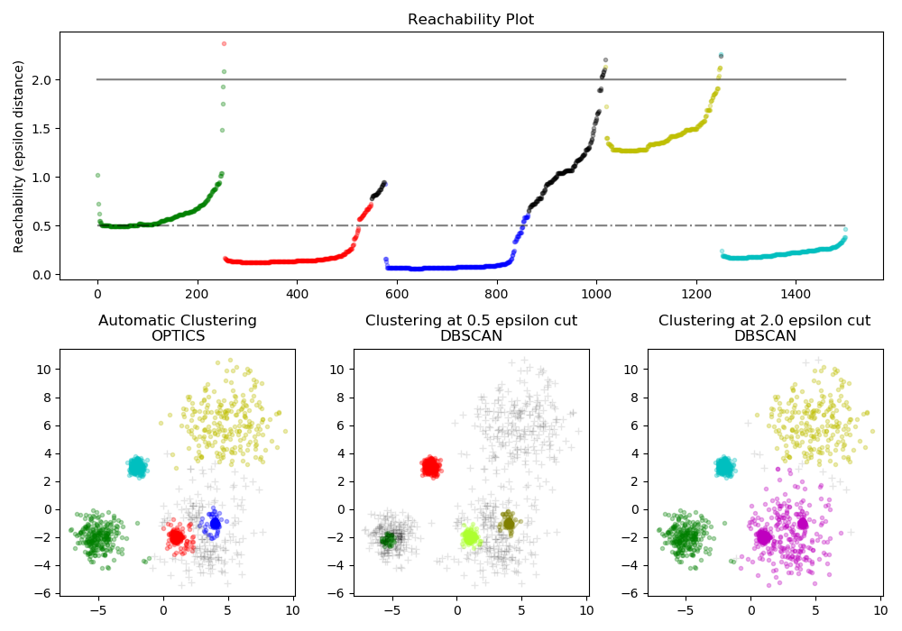
光学聚类算法的演示
发现高密度的核心样本并从中扩展聚类。此示例使用生成的数据,以使聚类具有不同的密度。sklearn.cluster.OPTICS首先与它的Xi聚类检测方法一起使用, 然后设置可达性的特定阈值, 这对应于sklearn.cluster.DBSCAN。我们可以看到,在DBSCAN中,通过不同的阈值选择,可以恢复不同的光学团簇的Xi方法。
# Authors: Shane Grigsby <refuge@rocktalus.com>
#          Adrin Jalali <adrin.jalali@gmail.com>
# License: BSD 3 clause


from sklearn.cluster import OPTICS, cluster_optics_dbscan
import matplotlib.gridspec as gridspec
import matplotlib.pyplot as plt
import numpy as np

# Generate sample data

np.random.seed(0)
n_points_per_cluster = 250

C1 = [-5, -2] + .8 * np.random.randn(n_points_per_cluster, 2)
C2 = [4, -1] + .1 * np.random.randn(n_points_per_cluster, 2)
C3 = [1, -2] + .2 * np.random.randn(n_points_per_cluster, 2)
C4 = [-2, 3] + .3 * np.random.randn(n_points_per_cluster, 2)
C5 = [3, -2] + 1.6 * np.random.randn(n_points_per_cluster, 2)
C6 = [5, 6] + 2 * np.random.randn(n_points_per_cluster, 2)
X = np.vstack((C1, C2, C3, C4, C5, C6))

clust = OPTICS(min_samples=50, xi=.05, min_cluster_size=.05)

# Run the fit
clust.fit(X)

labels_050 = cluster_optics_dbscan(reachability=clust.reachability_,
                                   core_distances=clust.core_distances_,
                                   ordering=clust.ordering_, eps=0.5)
labels_200 = cluster_optics_dbscan(reachability=clust.reachability_,
                                   core_distances=clust.core_distances_,
                                   ordering=clust.ordering_, eps=2)

space = np.arange(len(X))
reachability = clust.reachability_[clust.ordering_]
labels = clust.labels_[clust.ordering_]

plt.figure(figsize=(10, 7))
G = gridspec.GridSpec(2, 3)
ax1 = plt.subplot(G[0, :])
ax2 = plt.subplot(G[1, 0])
ax3 = plt.subplot(G[1, 1])
ax4 = plt.subplot(G[1, 2])

# Reachability plot
colors = ['g.', 'r.', 'b.', 'y.', 'c.']
for klass, color in zip(range(0, 5), colors):
    Xk = space[labels == klass]
    Rk = reachability[labels == klass]
    ax1.plot(Xk, Rk, color, alpha=0.3)
ax1.plot(space[labels == -1], reachability[labels == -1], 'k.', alpha=0.3)
ax1.plot(space, np.full_like(space, 2., dtype=float), 'k-', alpha=0.5)
ax1.plot(space, np.full_like(space, 0.5, dtype=float), 'k-.', alpha=0.5)
ax1.set_ylabel('Reachability (epsilon distance)')
ax1.set_title('Reachability Plot')

# OPTICS
colors = ['g.', 'r.', 'b.', 'y.', 'c.']
for klass, color in zip(range(0, 5), colors):
    Xk = X[clust.labels_ == klass]
    ax2.plot(Xk[:, 0], Xk[:, 1], color, alpha=0.3)
ax2.plot(X[clust.labels_ == -1, 0], X[clust.labels_ == -1, 1], 'k+', alpha=0.1)
ax2.set_title('Automatic Clustering\nOPTICS')

# DBSCAN at 0.5
colors = ['g', 'greenyellow', 'olive', 'r', 'b', 'c']
for klass, color in zip(range(0, 6), colors):
    Xk = X[labels_050 == klass]
    ax3.plot(Xk[:, 0], Xk[:, 1], color, alpha=0.3, marker='.')
ax3.plot(X[labels_050 == -1, 0], X[labels_050 == -1, 1], 'k+', alpha=0.1)
ax3.set_title('Clustering at 0.5 epsilon cut\nDBSCAN')

# DBSCAN at 2.
colors = ['g.', 'm.', 'y.', 'c.']
for klass, color in zip(range(0, 4), colors):
    Xk = X[labels_200 == klass]
    ax4.plot(Xk[:, 0], Xk[:, 1], color, alpha=0.3)
ax4.plot(X[labels_200 == -1, 0], X[labels_200 == -1, 1], 'k+', alpha=0.1)
ax4.set_title('Clustering at 2.0 epsilon cut\nDBSCAN')

plt.tight_layout()
plt.show()
脚本的总运行时间:(0分1.520秒)

