sklearn.discriminant_analysis.LinearDiscriminantAnalysis
class sklearn.discriminant_analysis.LinearDiscriminantAnalysis(*, solver='svd', shrinkage=None, priors=None, n_components=None, store_covariance=False, tol=0.0001)
线性判别分析
利用贝叶斯规则对数据拟合类条件密度,生成具有线性判定边界的分类器。
该模型对每个类拟合一个高斯密度,假设所有类有相同的协方差矩阵。
拟合模型还可以利用 transform方法将输入投影到最具辨别力的方向,从而降低输入的维数。
0.17版本新增:LinearDiscriminantAnalysis。
在用户指南中获取更多内容。
| 参数 | 说明 |
|---|---|
| solver | {"svd","lsqr","eigen"}, default = "svd" 解算器可能使用的值: ♦"svd": 奇异值分解(默认)。不计算协方差矩阵,因此该解算器被推荐用于具有大量特征的数据。 ♦"lsqr": 最小二乘解,能够与收缩参数合并使用。 ♦"eigen": 特征值分解,能够与收缩参数合并使用。 |
| shrinkage | "auto" or float,default = None 收缩参数可能使用的值: ♦None: 无收缩(默认)。 ♦"auto": 利用Ledoit-Wolf引理进行自动收缩。 ♦float between 0 and1: 0 到 1 之间的修正收缩参数。 注意,收缩参数仅在"lsqr"和"eigen"解算器中有效。 |
| priors | Array_like of shape (n_classes,), default = None 先验概率。默认情况下,类的比例是根据训练集推断出来的。 |
| n_components | int, default = None 降维所保留的成分个数(<= min(n_classed - 1, n_features))。如果为None,该值会赋予min(n_classes - 1, n_features)。该参数值会对变化方法产生影响。 |
| store_convariance | bool, default = False 若为真,当解算器为"svd"时,明确计算加权的类内协方差矩阵。不论真/假,其余两种解算器的矩阵总是会被计算并储存。 0.17版本新增。 |
| tol | float, default = 1.0e-4 对于X一个奇异值的绝对阈值,常常被用来估计X的秩,这种估计是显著的。仅当解算器为"svd"时,不显著的奇异值维度将会被舍弃。 0.17版本新增。 |
| 属性 | 说明 |
|---|---|
| chef_ | ndarray of shape (n_features,) or (n_classes, n_features) 权重向量。 |
| intercept_ | ndarray of shape (n_classes,) 截距项。 |
| covariance_ | array-like of shape(n_features, n_features) 加权类内协方差矩阵。它对应于sum_k prior_k * C_k,其中C_k是k类样本的协方差矩阵,同时它也是个估计量,来源于(可能缩小的)协方差的有偏估计。如果解算器为"svd",该矩阵仅在store_convariance = True的情况下存在。 |
| explained_variance_ratio_ | ndarray of shape (n_components,) 每个被选中成分所能解释的方差的百分比。如果n_conponents这个参数没有被设置,那么所有的成分都将被保存,同时所有解释方差的累积之和会等于1。 该值只有在"eigen" 或"svd"两解算器情况下可以得到。 |
| means_ | array-like of shape (n_classes, n_features) "类"均值。 |
| priors_ | array_like of shape (n_classes,) 类先验(和为1)。 |
| scalings_ | array-like of shape (rank, n_classes - 1) 缩放特征存在于由类心所张成的空间之中。仅可以在解算器为"svd" 和"eigen"情况下获得。 |
| xbar_ | array-like of shape (n_features,) 整体均值。只有在解算器为"svd"时,会予以展示。 |
| classes_ | array-like of shape (n_classes) 唯一类标签。 |
另见:
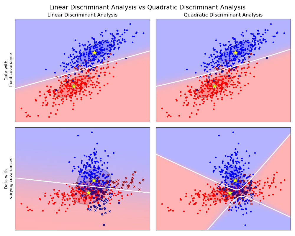
sklearn.discriminant_analysis.QuadraticDiscriminantAnalysis二次判别分析
示例:
>>> import numpy as np
>>> from sklearn.discriminant_analysis import LinearDiscriminantAnalysis
>>> X = np.array([[-1, -1], [-2, -1], [-3, -2], [1, 1], [2, 1], [3, 2]])
>>> y = np.array([1, 1, 1, 2, 2, 2])
>>> clf = LinearDiscriminantAnalysis()
>>> clf.fit(X, y)
LinearDiscriminantAnalysis()
>>> print(clf.predict([[-0.8, -1]]))
[1]
方法
| 方法 | 说明 |
|---|---|
decision_function(self, X) |
将决策函数应用于样本数组 |
fit(self, X, y) |
根据给定的模型拟合LinearDiscriminantAnalysis模型 |
fit_transform(self, X[, y]) |
拟合数据然后将其进行转化 |
get_params(self[, deep]) |
获取当前估计量的参数 |
predict(self, X) |
预测X中的样本类型标签 |
predict_log_proba(self, X) |
估计对数概率 |
predict_proba(self, X) |
估计概率 |
score(self, X, y[, sample_weight]) |
返回给定测试数据和标签的平均精度 |
set_params(self, **params) |
设置当前估计量的参数 |
transform(self, X) |
将数据投射至最大类分块中 |
__init__(self, *, solver='svd', shrinkage=None, priors=None, n_components=None, store_covariance=False, tol=0.0001)
初始化self。请参阅help(type(self))以获得准确的说明。
decision_function(self, X)
对一个样本数组应用决策函数。
决策函数等于(取决于一个常数向量)模型的对数后验概率,也就是,log p(y = k | x)。在二元分类中,作出如下设置来对应区别。log p(y = 1 | x) - log p(y = 0 | x)。参见 LDA和QDA分类器的数学公式。
| 参数 | 说明 |
|---|---|
| X | array-like of shape (n_samples, n_features) 样本数组(测试向量)。 |
| 返回值 | 说明 |
|---|---|
| C | ndarray of shape (n_samples,) or (n_sample, n_classes) 决策函数值与每个类、样本相关。在二分类的样例中,样本大小为(n_samples, ),给出正类的对数似然比。 |
fit(self, X, y)
根据给定的模型拟合LinearDiscriminantAnalysis模型
训练数据及参数。
0.19版本更变:store_covariance被移至主要构造函数
tol被移至主要构造函数
| 参数 | 说明 |
|---|---|
| X | array-like of shape (n_samples, n_features) 训练数据 |
| y | array-like of shape (n_sample, ) 目标值 |
fit_transform(self, X, y=None, fit_params)
拟合数据然后将其进行转化。
使用可选参数fit_params将转换器拟合到X和y,并返回X的转换值。
| 参数 | 说明 |
|---|---|
| X | {array-like, sparse matrix, dataframe} of shape (n_sample, n_features) |
| y | ndarray of shape (n_samples, ), default = None 目标值 |
| **fit_params | dict 附加拟合参数 |
| 返回值 | 说明 |
|---|---|
| X_new | ndarray array of shape (n_samples, n_features_new) 转化后的数组 |
get_params(self, deep=True)
获取当前估计量的参数
| 参数 | 说明 |
|---|---|
| deep | bool, default = True 如果为真,则将返回此估计器和其所包含子对象的参数 |
| 返回值 | 说明 |
|---|---|
| params | mapping of string to any 参数名被映射至他们的值 |
predict(self, X)
预测X中的样本类型标签。
| 参数 | 说明 |
|---|---|
| X | array_like or sparse matrix, shape (n_samples, n_features) 样本 |
| 返回值 | 说明 |
|---|---|
| C | array, shape [n_samples] 每个样本所获得预测的分类标签 |
predict_log_proba(self, X)
估计对数概率
| 参数 | 说明 |
|---|---|
| X | array-like of shape (n_sample, n_features) 输入数据 |
| 返回值 | 说明 |
|---|---|
| C | ndarray of shape (n_sample, n_classes) 估计后的对数概率 |
predict_proba(self, X)
估计概率
| 参数 | 说明 |
|---|---|
| X | array-like of shape (n_sample, n_features) 输入数据 |
| 返回值 | 说明 |
|---|---|
| C | ndarray of shape (n_sample, n_classes) 估计后的对数概率 |
score(self, X, y, sample_weight=None)
返回给定测试数据和标签的平均精度。
在多标签分类中,这是子集准确性,这是一个严格的指标,因为你需要对每个样本正确预测每个标签集。
| 参数 | 说明 |
|---|---|
| X | array-like of sshape (n_samples, nfeatures) 测试样本 |
| y | array-like of shape (n_sample, ) or (n_samples, n_outputs) X中结果为真的标签 |
| 返回值 | 说明 |
|---|---|
| score | float self.predict(X) wrt. y.的平均精度 |
set_params(self, **params)
设置当前估计量的参数。
该方法适用于简单估计量和嵌套对象(如pipline)。后者具有形式为<component>_<parameter>的参数,这样就让更新嵌套对象的每个组件成为了可能。
| 参数 | 说明 |
|---|---|
| f_params | dict 估计量参数 |
| 返回值 | 说明 |
|---|---|
| self | object 估计器实例 |
transform(self, X)
将数据投射至最大类分块中。
| 参数 | 说明 |
|---|---|
| X | array-like of shape (n_samples, n_features) 输入数据 |
| 返回值 | 说明 |
|---|---|
| X_new | ndarray of shape (n_samples, n_features) 转换后的数据 |