

手写数字上的流形学习:局部线性嵌入,Isomap…
现在来看数字数据集上各种嵌入的说明。
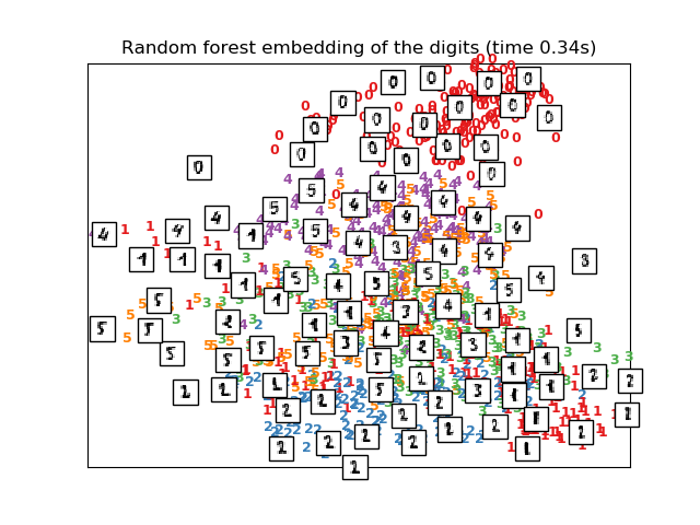
RandomTreesEmbedding,来自 sklearn.ensemble模块, 在技术上不是一种流形嵌入方法,因为它学习了一种高维表示,我们在其上应用了一种降维方法。但是,将数据集转换为类是线性可分的表示, 这通常是有用的。
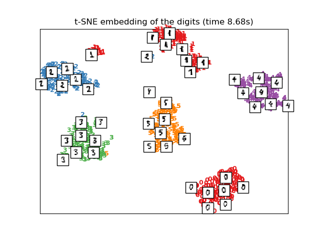
在本例中,T-SNE将使用PCA生成的嵌入进行初始化,这不是默认设置。它保证了嵌入的全局稳定性,即嵌入不依赖于随机初始化。
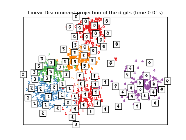
线性判别分析, 来自sklearn.discriminant_analysis模块 、和邻域成分分析, 来自sklearn.neighbors模块, 是一种有监督的降维方法,即利用所提供的标签,而不是其他方法。


Computing random projection
Computing PCA projection
Computing Linear Discriminant Analysis projection
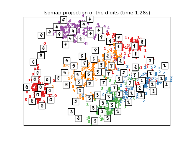
Computing Isomap projection
Done.
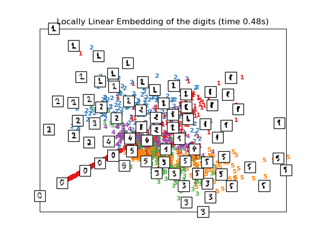
Computing LLE embedding
Done. Reconstruction error: 1.63544e-06
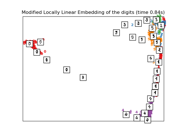
Computing modified LLE embedding
Done. Reconstruction error: 0.360613
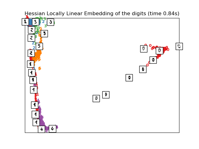
Computing Hessian LLE embedding
Done. Reconstruction error: 0.212803
Computing LTSA embedding
Done. Reconstruction error: 0.212804
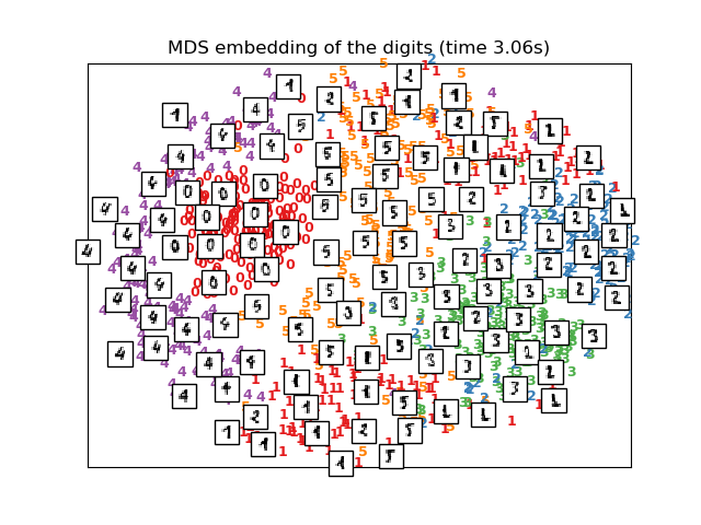
Computing MDS embedding
Done. Stress: 174889755.062254
Computing Totally Random Trees embedding
Computing Spectral embedding
Computing t-SNE embedding
Computing NCA projection
# Authors: Fabian Pedregosa <fabian.pedregosa@inria.fr>
# Olivier Grisel <olivier.grisel@ensta.org>
# Mathieu Blondel <mathieu@mblondel.org>
# Gael Varoquaux
# License: BSD 3 clause (C) INRIA 2011
from time import time
import numpy as np
import matplotlib.pyplot as plt
from matplotlib import offsetbox
from sklearn import (manifold, datasets, decomposition, ensemble,
discriminant_analysis, random_projection, neighbors)
print(__doc__)
digits = datasets.load_digits(n_class=6)
X = digits.data
y = digits.target
n_samples, n_features = X.shape
n_neighbors = 30
# ----------------------------------------------------------------------
# Scale and visualize the embedding vectors
def plot_embedding(X, title=None):
x_min, x_max = np.min(X, 0), np.max(X, 0)
X = (X - x_min) / (x_max - x_min)
plt.figure()
ax = plt.subplot(111)
for i in range(X.shape[0]):
plt.text(X[i, 0], X[i, 1], str(y[i]),
color=plt.cm.Set1(y[i] / 10.),
fontdict={'weight': 'bold', 'size': 9})
if hasattr(offsetbox, 'AnnotationBbox'):
# only print thumbnails with matplotlib > 1.0
shown_images = np.array([[1., 1.]]) # just something big
for i in range(X.shape[0]):
dist = np.sum((X[i] - shown_images) ** 2, 1)
if np.min(dist) < 4e-3:
# don't show points that are too close
continue
shown_images = np.r_[shown_images, [X[i]]]
imagebox = offsetbox.AnnotationBbox(
offsetbox.OffsetImage(digits.images[i], cmap=plt.cm.gray_r),
X[i])
ax.add_artist(imagebox)
plt.xticks([]), plt.yticks([])
if title is not None:
plt.title(title)
# ----------------------------------------------------------------------
# Plot images of the digits
n_img_per_row = 20
img = np.zeros((10 * n_img_per_row, 10 * n_img_per_row))
for i in range(n_img_per_row):
ix = 10 * i + 1
for j in range(n_img_per_row):
iy = 10 * j + 1
img[ix:ix + 8, iy:iy + 8] = X[i * n_img_per_row + j].reshape((8, 8))
plt.imshow(img, cmap=plt.cm.binary)
plt.xticks([])
plt.yticks([])
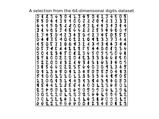
plt.title('A selection from the 64-dimensional digits dataset')
# ----------------------------------------------------------------------
# Random 2D projection using a random unitary matrix
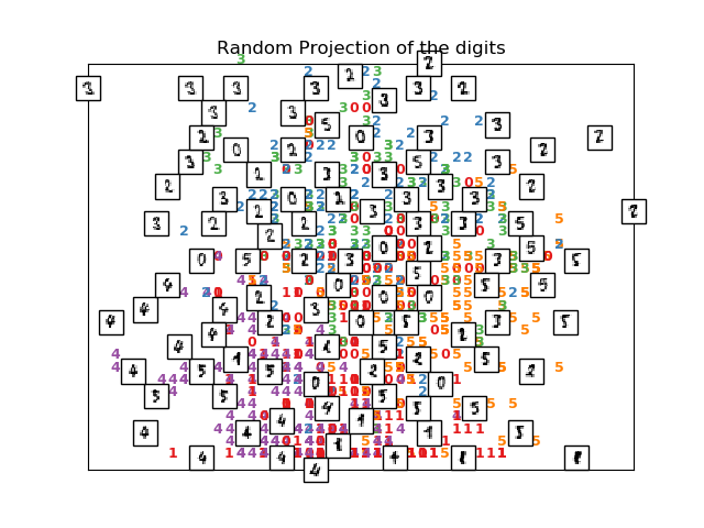
print("Computing random projection")
rp = random_projection.SparseRandomProjection(n_components=2, random_state=42)
X_projected = rp.fit_transform(X)
plot_embedding(X_projected, "Random Projection of the digits")
# ----------------------------------------------------------------------
# Projection on to the first 2 principal components
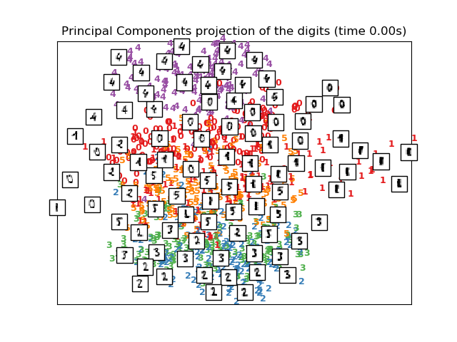
print("Computing PCA projection")
t0 = time()
X_pca = decomposition.TruncatedSVD(n_components=2).fit_transform(X)
plot_embedding(X_pca,
"Principal Components projection of the digits (time %.2fs)" %
(time() - t0))
# ----------------------------------------------------------------------
# Projection on to the first 2 linear discriminant components
print("Computing Linear Discriminant Analysis projection")
X2 = X.copy()
X2.flat[::X.shape[1] + 1] += 0.01 # Make X invertible
t0 = time()
X_lda = discriminant_analysis.LinearDiscriminantAnalysis(n_components=2
).fit_transform(X2, y)
plot_embedding(X_lda,
"Linear Discriminant projection of the digits (time %.2fs)" %
(time() - t0))
# ----------------------------------------------------------------------
# Isomap projection of the digits dataset
print("Computing Isomap projection")
t0 = time()
X_iso = manifold.Isomap(n_neighbors=n_neighbors, n_components=2
).fit_transform(X)
print("Done.")
plot_embedding(X_iso,
"Isomap projection of the digits (time %.2fs)" %
(time() - t0))
# ----------------------------------------------------------------------
# Locally linear embedding of the digits dataset
print("Computing LLE embedding")
clf = manifold.LocallyLinearEmbedding(n_neighbors=n_neighbors, n_components=2,
method='standard')
t0 = time()
X_lle = clf.fit_transform(X)
print("Done. Reconstruction error: %g" % clf.reconstruction_error_)
plot_embedding(X_lle,
"Locally Linear Embedding of the digits (time %.2fs)" %
(time() - t0))
# ----------------------------------------------------------------------
# Modified Locally linear embedding of the digits dataset
print("Computing modified LLE embedding")
clf = manifold.LocallyLinearEmbedding(n_neighbors=n_neighbors, n_components=2,
method='modified')
t0 = time()
X_mlle = clf.fit_transform(X)
print("Done. Reconstruction error: %g" % clf.reconstruction_error_)
plot_embedding(X_mlle,
"Modified Locally Linear Embedding of the digits (time %.2fs)" %
(time() - t0))
# ----------------------------------------------------------------------
# HLLE embedding of the digits dataset
print("Computing Hessian LLE embedding")
clf = manifold.LocallyLinearEmbedding(n_neighbors=n_neighbors, n_components=2,
method='hessian')
t0 = time()
X_hlle = clf.fit_transform(X)
print("Done. Reconstruction error: %g" % clf.reconstruction_error_)
plot_embedding(X_hlle,
"Hessian Locally Linear Embedding of the digits (time %.2fs)" %
(time() - t0))
# ----------------------------------------------------------------------
# LTSA embedding of the digits dataset
print("Computing LTSA embedding")
clf = manifold.LocallyLinearEmbedding(n_neighbors=n_neighbors, n_components=2,
method='ltsa')
t0 = time()
X_ltsa = clf.fit_transform(X)
print("Done. Reconstruction error: %g" % clf.reconstruction_error_)
plot_embedding(X_ltsa,
"Local Tangent Space Alignment of the digits (time %.2fs)" %
(time() - t0))
# ----------------------------------------------------------------------
# MDS embedding of the digits dataset
print("Computing MDS embedding")
clf = manifold.MDS(n_components=2, n_init=1, max_iter=100)
t0 = time()
X_mds = clf.fit_transform(X)
print("Done. Stress: %f" % clf.stress_)
plot_embedding(X_mds,
"MDS embedding of the digits (time %.2fs)" %
(time() - t0))
# ----------------------------------------------------------------------
# Random Trees embedding of the digits dataset
print("Computing Totally Random Trees embedding")
hasher = ensemble.RandomTreesEmbedding(n_estimators=200, random_state=0,
max_depth=5)
t0 = time()
X_transformed = hasher.fit_transform(X)
pca = decomposition.TruncatedSVD(n_components=2)
X_reduced = pca.fit_transform(X_transformed)
plot_embedding(X_reduced,
"Random forest embedding of the digits (time %.2fs)" %
(time() - t0))
# ----------------------------------------------------------------------
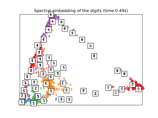
# Spectral embedding of the digits dataset
print("Computing Spectral embedding")
embedder = manifold.SpectralEmbedding(n_components=2, random_state=0,
eigen_solver="arpack")
t0 = time()
X_se = embedder.fit_transform(X)
plot_embedding(X_se,
"Spectral embedding of the digits (time %.2fs)" %
(time() - t0))
# ----------------------------------------------------------------------
# t-SNE embedding of the digits dataset
print("Computing t-SNE embedding")
tsne = manifold.TSNE(n_components=2, init='pca', random_state=0)
t0 = time()
X_tsne = tsne.fit_transform(X)
plot_embedding(X_tsne,
"t-SNE embedding of the digits (time %.2fs)" %
(time() - t0))
# ----------------------------------------------------------------------
# NCA projection of the digits dataset
print("Computing NCA projection")
nca = neighbors.NeighborhoodComponentsAnalysis(init='random',
n_components=2, random_state=0)
t0 = time()
X_nca = nca.fit_transform(X, y)
plot_embedding(X_nca,
"NCA embedding of the digits (time %.2fs)" %
(time() - t0))
plt.show()
脚本的总运行时间:(0分38.436秒)

