sklearn.linear_model.lasso_path
sklearn.linear_model.lasso_path(X, y, *, eps=0.001, n_alphas=100, alphas=None, precompute='auto', Xy=None, copy_X=True, coef_init=None, verbose=False, return_n_iter=False, positive=False, **params)
[源码]
计算具有坐标下降的套索路径
套索优化功能针对单输出和多输出而变化。
对于单输出任务,它是:
对于多输出任务,它是:
其中:
即每一行的范数之和。
在用户指南中阅读更多内容。
| 参数 | 返回值 |
|---|---|
| X | {array-like, sparse matrix} of shape (n_samples, n_features) 用于训练的数据。直接作为Fortran-contiguous数据传递,避免不必要的内存重复。如果 y是单输出,则X 可以是稀疏的。 |
| y | {array-like, sparse matrix} of shape (n_samples,) or (n_samples, n_outputs) 目标值 |
| eps | float, default=1e-3 路径的长度。 eps=1e-3意思是 alpha_min / alpha_max = 1e-3 |
| n_alphas | int, default=100 正则化路径中的Alpha数 |
| alphas | ndarray, default=None 用于在其中计算模型的alpha列表。如果为None,则自动设置Alpha。 |
| precompute | ‘auto’, bool or array-like of shape (n_features, n_features), default=’auto’ 是否使用预先计算的Gram矩阵来加快计算速度。如果设置 'auto'让我们决定。Gram矩阵也可以作为参数被传递。 |
| Xy | array-like of shape (n_features,) or (n_features, n_outputs), default=None 可以预先计算Xy = np.dot(XT,y)。仅当预先计算了Gram矩阵时才有用。 |
| copy_X | bool, default=True 如果为 True,将复制X;否则,它可能会被覆盖。 |
| coef_init | ndarray of shape (n_features, ), default=None 系数的初始值。 |
| verbose | bool or int, default=False 详细程度。 |
| return_n_iter | bool, default=False 是否返回迭代次数。 |
| positive | bool, default=False 如果设置为True,则强制系数为正。(仅当 y.ndim == 1时允许)。 |
| **params | kwargs 关键字参数传递给坐标下降求解器。 |
| 返回值 | 说明 |
|---|---|
| alphas | ndarray of shape (n_alphas,) 沿模型计算路径的Alpha。 |
| coefs | ndarray of shape (n_features, n_alphas) or (n_outputs, n_features, n_alphas) 沿路径的系数。 |
| dual_gaps | ndarray of shape (n_alphas,) 每个alpha优化结束时的双重间隔。 |
| n_iters | list of int 坐标下降优化器为达到每个alpha的指定公差所进行的迭代次数。 |
另见:
注
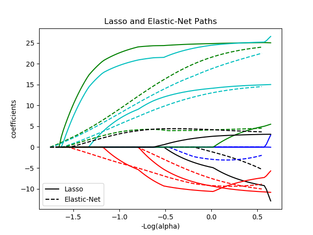
有关示例,请参阅examples / linear_model / plot_lasso_coordinate_descent_path.py。
为避免不必要的内存重复,fit方法的X参数应作为 Fortran-contiguous的numpy数组直接被传递。
请注意,在某些情况下,Lars求解器可能会更快地实现这个功能。特别是,线性插值可用于检索lars_path输出值之间的模型系数。
示例
将lasso_path和lars_path与插值进行比较:
>>> X = np.array([[1, 2, 3.1], [2.3, 5.4, 4.3]]).T
>>> y = np.array([1, 2, 3.1])
>>> # Use lasso_path to compute a coefficient path
>>> _, coef_path, _ = lasso_path(X, y, alphas=[5., 1., .5])
>>> print(coef_path)
[[0.         0.         0.46874778]
 [0.2159048  0.4425765  0.23689075]]
>>> # Now use lars_path and 1D linear interpolation to compute the
>>> # same path
>>> from sklearn.linear_model import lars_path
>>> alphas, active, coef_path_lars = lars_path(X, y, method='lasso')
>>> from scipy import interpolate
>>> coef_path_continuous = interpolate.interp1d(alphas[::-1],
...                                             coef_path_lars[:, ::-1])
>>> print(coef_path_continuous([5., 1., .5]))
[[0.         0.         0.46915237]
 [0.2159048  0.4425765  0.23668876]]