基于贝叶斯岭回归的曲线拟合¶

计算正弦波的贝叶斯岭回归。

有关回归的更多信息，请参见 Bayesian Ridge Regression。

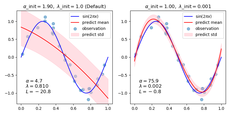
一般来说，在用贝叶斯岭回归拟合多项式曲线时，正则化参数(α，lambda)的初始值的选择可能是重要的。这是因为正则化参数是由依赖于初始值的迭代过程确定的。

在这个例子中，正弦波用多项式逼近，使用不同的初始值。

当从默认值(alpha_init=1.90，lambda_init=1.)开始时，结果曲线的偏差很大，而方差很小。因此，lambda_init应该设置相对较小的(1.e-3)，以减少偏差。

此外，通过评估这些模型的对数边际似然(L)，我们可以确定哪一种更好。可以得出结论，L较大的模型更有可能。

print(__doc__)

# Author: Yoshihiro Uchida <nimbus1after2a1sun7shower@gmail.com>

import numpy as np
import matplotlib.pyplot as plt

from sklearn.linear_model import BayesianRidge


def func(x): return np.sin(2*np.pi*x)


# #############################################################################
# Generate sinusoidal data with noise
size = 25
rng = np.random.RandomState(1234)
x_train = rng.uniform(0., 1., size)
y_train = func(x_train) + rng.normal(scale=0.1, size=size)
x_test = np.linspace(0., 1., 100)


# #############################################################################
# Fit by cubic polynomial
n_order = 3
X_train = np.vander(x_train, n_order + 1, increasing=True)
X_test = np.vander(x_test, n_order + 1, increasing=True)

# #############################################################################
# Plot the true and predicted curves with log marginal likelihood (L)
reg = BayesianRidge(tol=1e-6, fit_intercept=False, compute_score=True)
fig, axes = plt.subplots(1, 2, figsize=(8, 4))
for i, ax in enumerate(axes):
    # Bayesian ridge regression with different initial value pairs
    if i == 0:
        init = [1 / np.var(y_train), 1.]  # Default values
    elif i == 1:
        init = [1., 1e-3]
        reg.set_params(alpha_init=init[0], lambda_init=init[1])
    reg.fit(X_train, y_train)
    ymean, ystd = reg.predict(X_test, return_std=True)

    ax.plot(x_test, func(x_test), color="blue", label="sin($2\\pi x$)")
    ax.scatter(x_train, y_train, s=50, alpha=0.5, label="observation")
    ax.plot(x_test, ymean, color="red", label="predict mean")
    ax.fill_between(x_test, ymean-ystd, ymean+ystd,
                    color="pink", alpha=0.5, label="predict std")
    ax.set_ylim(-1.3, 1.3)
    ax.legend()
    title = "$\\alpha$_init$={:.2f},\\ \\lambda$_init$={}$".format(
            init[0], init[1])
    if i == 0:
        title += " (Default)"
    ax.set_title(title, fontsize=12)
    text = "$\\alpha={:.1f}$\n$\\lambda={:.3f}$\n$L={:.1f}$".format(
           reg.alpha_, reg.lambda_, reg.scores_[-1])
    ax.text(0.05, -1.0, text, fontsize=12)

plt.tight_layout()
plt.show()

脚本的总运行时间：(0分0.252秒)

Download Python source code: plot_bayesian_ridge_curvefit.py

Download Jupyter notebook:plot_bayesian_ridge_curvefit.ipynb