

Theil-Sen回归
在合成数据集上计算Theil-Sen回归。
有关回归器的更多信息,请参见 Theil-Sen estimator: generalized-median-based estimator。
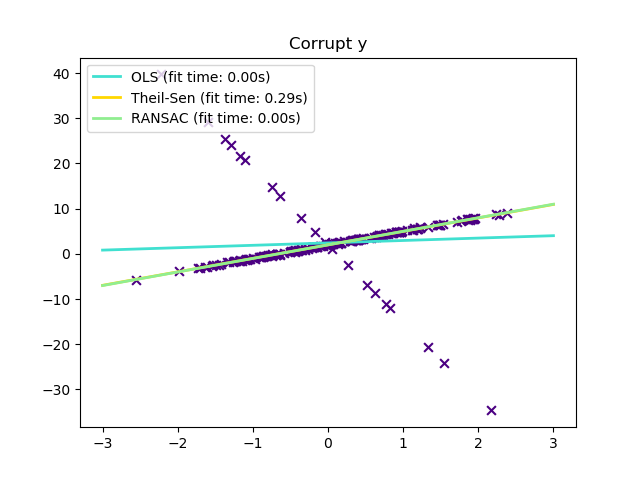
与OLS(普通最小二乘)估计相比,Theil-Sen估计对异常值具有较强的鲁棒性。在简单线性回归的情况下,它的崩溃点约为29.3%,这意味着它在二维情况下可以容忍任意损坏的数据(异常值)占比高达29.3%。
模型的估计是通过计算p子样本点的所有可能组合的子种群的斜率和截取来完成的。如果拟合了截距,则p必须大于或等于n_features + 1。最后的斜率和截距定义为这些斜率和截距的空间中值。
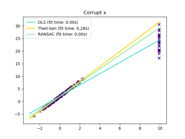
在某些情况下,Theil-Sen的性能优于 RANSAC,这也是一种很稳健的方法。这在下面的第二个例子中得到了说明,其中带异常值x轴扰动的RANSAC。调整RANSAC的 residual_threshold 参数可以弥补这一点,但是一般来说,需要对数据和异常值的性质有一个先验的了解。由于Theil-Sen计算的复杂性,建议只在样本数量和特征方面的小问题上使用它。对于较大的问题, max_subpopulation 参数将p子样本点的所有可能组合的大小限制为随机选择的子集,因此也限制了运行时。因此,Theil-Sen适用于较大的问题,其缺点是失去了它的一些数学性质,因为它是在随机子集上工作的。
# Author: Florian Wilhelm -- <florian.wilhelm@gmail.com>
# License: BSD 3 clause

import time
import numpy as np
import matplotlib.pyplot as plt
from sklearn.linear_model import LinearRegression, TheilSenRegressor
from sklearn.linear_model import RANSACRegressor

print(__doc__)

estimators = [('OLS', LinearRegression()),
              ('Theil-Sen', TheilSenRegressor(random_state=42)),
              ('RANSAC', RANSACRegressor(random_state=42)), ]
colors = {'OLS': 'turquoise', 'Theil-Sen': 'gold', 'RANSAC': 'lightgreen'}
lw = 2

# #############################################################################
# Outliers only in the y direction

np.random.seed(0)
n_samples = 200
# Linear model y = 3*x + N(2, 0.1**2)
x = np.random.randn(n_samples)
w = 3.
c = 2.
noise = 0.1 * np.random.randn(n_samples)
y = w * x + c + noise
# 10% outliers
y[-20:] += -20 * x[-20:]
X = x[:, np.newaxis]

plt.scatter(x, y, color='indigo', marker='x', s=40)
line_x = np.array([-3, 3])
for name, estimator in estimators:
    t0 = time.time()
    estimator.fit(X, y)
    elapsed_time = time.time() - t0
    y_pred = estimator.predict(line_x.reshape(2, 1))
    plt.plot(line_x, y_pred, color=colors[name], linewidth=lw,
             label='%s (fit time: %.2fs)' % (name, elapsed_time))

plt.axis('tight')
plt.legend(loc='upper left')
plt.title("Corrupt y")

# #############################################################################
# Outliers in the X direction

np.random.seed(0)
# Linear model y = 3*x + N(2, 0.1**2)
x = np.random.randn(n_samples)
noise = 0.1 * np.random.randn(n_samples)
y = 3 * x + 2 + noise
# 10% outliers
x[-20:] = 9.9
y[-20:] += 22
X = x[:, np.newaxis]

plt.figure()
plt.scatter(x, y, color='indigo', marker='x', s=40)

line_x = np.array([-3, 10])
for name, estimator in estimators:
    t0 = time.time()
    estimator.fit(X, y)
    elapsed_time = time.time() - t0
    y_pred = estimator.predict(line_x.reshape(2, 1))
    plt.plot(line_x, y_pred, color=colors[name], linewidth=lw,
             label='%s (fit time: %.2fs)' % (name, elapsed_time))

plt.axis('tight')
plt.legend(loc='upper left')
plt.title("Corrupt x")
plt.show()
脚本的总运行时间:(0分0.749秒)。

