梯度提升回归¶

此示例演示了梯度提升从一组弱预测模型生成预测模型。梯度提升可以用于回归和分类问题。在这里，我们将训练一个模型来处理糖尿病回归任务。我们将从梯度提升回归器中得到结果， 这个梯度提升回归器是使用最小二乘损失， 和500课深度为4的回归树组成。

注：对于较大的数据集(n_samples >= 10000)，请参阅sklearn.ensemble.HistGradientBoostingRegressor。

print(__doc__)

# Author: Peter Prettenhofer <peter.prettenhofer@gmail.com>
#         Maria Telenczuk <https://github.com/maikia>
#         Katrina Ni <https://github.com/nilichen>
#
# License: BSD 3 clause

import matplotlib.pyplot as plt
import numpy as np
from sklearn import datasets, ensemble
from sklearn.inspection import permutation_importance
from sklearn.metrics import mean_squared_error
from sklearn.model_selection import train_test_split

加载数据

首先，我们需要加载数据。

diabetes = datasets.load_diabetes()
X, y = diabetes.data, diabetes.target

数据预处理

接下来，我们将我们的数据集分割成90%用于训练，剩下的用作测试。我们还将设置回归模型的参数。您可以使用这些参数查看结果如何变化。

n_estimators :将执行的提升次数。稍后，我们将绘制反提升迭代的偏差。

max_depth :限制树中的节点数。最佳的值取决于输入变量之间的相互作用。

min_samples_split :内部节点分割时所需的最小样本数。

learning_rate :每棵树的贡献会减少多少。

loss :损失函数优化。在这种情况下，使用最小二乘函数，但是还有许多其他选项。(看GradientBoostingRegressor)。

X_train, X_test, y_train, y_test = train_test_split(
    X, y, test_size=0.1, random_state=13)

params = {'n_estimators': 500,
          'max_depth': 4,
          'min_samples_split': 5,
          'learning_rate': 0.01,
          'loss': 'ls'}

拟合回归模型

现在，我们将初始化一个梯度提升回归器，并将其与我们的训练数据进行拟合。让我们也看看测试数据的均方误差。

reg = ensemble.GradientBoostingRegressor(**params)
reg.fit(X_train, y_train)

mse = mean_squared_error(y_test, reg.predict(X_test))
print("The mean squared error (MSE) on test set: {:.4f}".format(mse))

The mean squared error (MSE) on test set: 3017.9419

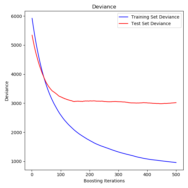
绘制训练偏差

最后，我们将可视化结果。要做到这一点，我们将首先计算测试集偏差，然后根据提升迭代绘制测试集偏差图。

test_score = np.zeros((params['n_estimators'],), dtype=np.float64)
for i, y_pred in enumerate(reg.staged_predict(X_test)):
    test_score[i] = reg.loss_(y_test, y_pred)

fig = plt.figure(figsize=(6, 6))
plt.subplot(1, 1, 1)
plt.title('Deviance')
plt.plot(np.arange(params['n_estimators']) + 1, reg.train_score_, 'b-',
         label='Training Set Deviance')
plt.plot(np.arange(params['n_estimators']) + 1, test_score, 'r-',
         label='Test Set Deviance')
plt.legend(loc='upper right')
plt.xlabel('Boosting Iterations')
plt.ylabel('Deviance')
fig.tight_layout()
plt.show()

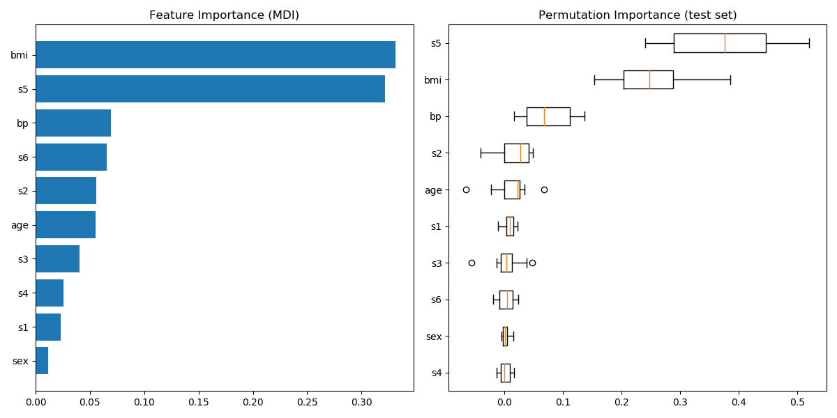
绘制特征重要性

小心一点、基于不纯度的特征重要性对于高基数的特征(许多唯一的值)可能会产生误导。作为一个替代项,reg的排列重要性可以在一个保持的测试集上计算。看Permutation feature importance更多细节。

在本例中，基于不纯度和排列方法识别相同的2个强预测特征，但顺序不同。第三大预测特征，“bp”，在这两种方法中也是相同的。其余特征的预测性较低，排列图中的错误条显示它们与0重叠。

feature_importance = reg.feature_importances_
sorted_idx = np.argsort(feature_importance)
pos = np.arange(sorted_idx.shape[0]) + .5
fig = plt.figure(figsize=(12, 6))
plt.subplot(1, 2, 1)
plt.barh(pos, feature_importance[sorted_idx], align='center')
plt.yticks(pos, np.array(diabetes.feature_names)[sorted_idx])
plt.title('Feature Importance (MDI)')

result = permutation_importance(reg, X_test, y_test, n_repeats=10,
                                random_state=42, n_jobs=2)
sorted_idx = result.importances_mean.argsort()
plt.subplot(1, 2, 2)
plt.boxplot(result.importances[sorted_idx].T,
            vert=False, labels=np.array(diabetes.feature_names)[sorted_idx])
plt.title("Permutation Importance (test set)")
fig.tight_layout()
plt.show()

脚本的总运行时间：(0分2.168秒)

Download Python source code:plot_gradient_boosting_regression.py

Download Jupyter notebook:plot_gradient_boosting_regression.ipynb