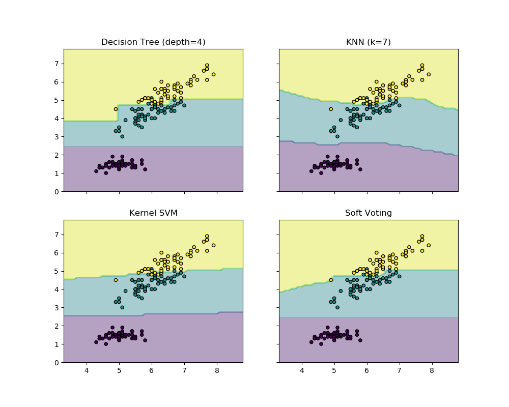
绘制投票分类器的决策边界¶

使用Iris数据集的两个特征绘制投票分类器的决策边界。

绘制toy数据集中第一个样本的类概率，由三个不同的分类器预测，并由VotingClassfier平均。

首先，初始化了三个示例性分类器(DecisionTreeClassifier,KNeighborsClassifier, 和 SVC)， 并且使用权重为[2, 1, 2]的软-投票VotingClassifier， 这意味着当计算平均概率时，DecisionTreeClassifier和 SVC的预测概率的权重是KNeighborsClassifier的权重的2倍。

print(__doc__)

from itertools import product

import numpy as np
import matplotlib.pyplot as plt

from sklearn import datasets
from sklearn.tree import DecisionTreeClassifier
from sklearn.neighbors import KNeighborsClassifier
from sklearn.svm import SVC
from sklearn.ensemble import VotingClassifier

# Loading some example data
iris = datasets.load_iris()
X = iris.data[:, [0, 2]]
y = iris.target

# Training classifiers
clf1 = DecisionTreeClassifier(max_depth=4)
clf2 = KNeighborsClassifier(n_neighbors=7)
clf3 = SVC(gamma=.1, kernel='rbf', probability=True)
eclf = VotingClassifier(estimators=[('dt', clf1), ('knn', clf2),
                                    ('svc', clf3)],
                        voting='soft', weights=[2, 1, 2])

clf1.fit(X, y)
clf2.fit(X, y)
clf3.fit(X, y)
eclf.fit(X, y)

# Plotting decision regions
x_min, x_max = X[:, 0].min() - 1, X[:, 0].max() + 1
y_min, y_max = X[:, 1].min() - 1, X[:, 1].max() + 1
xx, yy = np.meshgrid(np.arange(x_min, x_max, 0.1),
                     np.arange(y_min, y_max, 0.1))

f, axarr = plt.subplots(2, 2, sharex='col', sharey='row', figsize=(10, 8))

for idx, clf, tt in zip(product([0, 1], [0, 1]),
                        [clf1, clf2, clf3, eclf],
                        ['Decision Tree (depth=4)', 'KNN (k=7)',
                         'Kernel SVM', 'Soft Voting']):

    Z = clf.predict(np.c_[xx.ravel(), yy.ravel()])
    Z = Z.reshape(xx.shape)

    axarr[idx[0], idx[1]].contourf(xx, yy, Z, alpha=0.4)
    axarr[idx[0], idx[1]].scatter(X[:, 0], X[:, 1], c=y,
                                  s=20, edgecolor='k')
    axarr[idx[0], idx[1]].set_title(tt)

plt.show()

脚本的总运行时间：(0分0.462秒)

Download Python source code: plot_voting_decision_regions.py

Download Jupyter notebook:plot_voting_decision_regions.ipynb