

收缩协方差估计:LedoitWolf VS OAS和极大似然
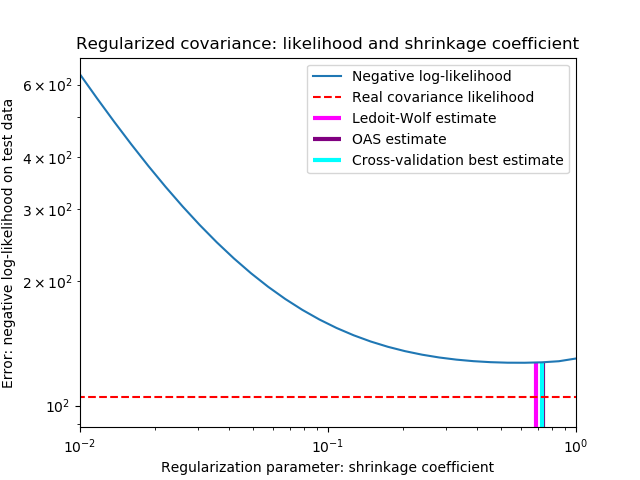
当处理协方差估计时,通常的方法是使用极大似然估计。例如 sklearn.covariance.EmpiricalCovariance,这是不偏不倚的。当给出许多观测结果时,它收敛到真实的(总体)协方差。然而,正则化也可能是有益的,以减少它的方差;这反过来又带来一些偏差。这个例子说明了在 Shrunk Covariance估计中使用的简单正则化。特别是如何设置正则化的数量,即如何选择偏差-方差权衡。
在这里,我们比较了三种方法:
根据潜在收缩参数的网格,通过三折交叉验证的可能性来设置参数。 Ledoit和Wolf提出的求渐近最优正则化参数(最小MSE准则)的封闭公式,得到了 sklearn.covariance.LedoitWolf协方差估计。关于 Ledoit-Wolf收缩的改进, sklearn.covariance.OAS,由Chen等人提出。在假设数据是高斯的情况下,特别是对于小样本,它的收敛性要好得多。
为了量化估计误差,我们对收缩参数的不同值绘制了不可见数据的可能性图。我们还通过LedoitWolf和OAS估计的交叉验证进行选择显示。
请注意,极大似然估计值没有收缩,因此表现不佳。Ledoit-Wolf估计的表现非常好,因为它接近最优,而且计算成本不高。在这个例子中,OAS的估计更远一点。有趣的是,这两种方法的性能都优于交叉验证,因为交叉验证在计算上开销最大。
print(__doc__)

import numpy as np
import matplotlib.pyplot as plt
from scipy import linalg

from sklearn.covariance import LedoitWolf, OAS, ShrunkCovariance, \
    log_likelihood, empirical_covariance
from sklearn.model_selection import GridSearchCV


# #############################################################################
# Generate sample data
n_features, n_samples = 40, 20
np.random.seed(42)
base_X_train = np.random.normal(size=(n_samples, n_features))
base_X_test = np.random.normal(size=(n_samples, n_features))

# Color samples
coloring_matrix = np.random.normal(size=(n_features, n_features))
X_train = np.dot(base_X_train, coloring_matrix)
X_test = np.dot(base_X_test, coloring_matrix)

# #############################################################################
# Compute the likelihood on test data

# spanning a range of possible shrinkage coefficient values
shrinkages = np.logspace(-2, 0, 30)
negative_logliks = [-ShrunkCovariance(shrinkage=s).fit(X_train).score(X_test)
                    for s in shrinkages]

# under the ground-truth model, which we would not have access to in real
# settings
real_cov = np.dot(coloring_matrix.T, coloring_matrix)
emp_cov = empirical_covariance(X_train)
loglik_real = -log_likelihood(emp_cov, linalg.inv(real_cov))

# #############################################################################
# Compare different approaches to setting the parameter

# GridSearch for an optimal shrinkage coefficient
tuned_parameters = [{'shrinkage': shrinkages}]
cv = GridSearchCV(ShrunkCovariance(), tuned_parameters)
cv.fit(X_train)

# Ledoit-Wolf optimal shrinkage coefficient estimate
lw = LedoitWolf()
loglik_lw = lw.fit(X_train).score(X_test)

# OAS coefficient estimate
oa = OAS()
loglik_oa = oa.fit(X_train).score(X_test)

# #############################################################################
# Plot results
fig = plt.figure()
plt.title("Regularized covariance: likelihood and shrinkage coefficient")
plt.xlabel('Regularization parameter: shrinkage coefficient')
plt.ylabel('Error: negative log-likelihood on test data')
# range shrinkage curve
plt.loglog(shrinkages, negative_logliks, label="Negative log-likelihood")

plt.plot(plt.xlim(), 2 * [loglik_real], '--r',
         label="Real covariance likelihood")

# adjust view
lik_max = np.amax(negative_logliks)
lik_min = np.amin(negative_logliks)
ymin = lik_min - 6. * np.log((plt.ylim()[1] - plt.ylim()[0]))
ymax = lik_max + 10. * np.log(lik_max - lik_min)
xmin = shrinkages[0]
xmax = shrinkages[-1]
# LW likelihood
plt.vlines(lw.shrinkage_, ymin, -loglik_lw, color='magenta',
           linewidth=3, label='Ledoit-Wolf estimate')
# OAS likelihood
plt.vlines(oa.shrinkage_, ymin, -loglik_oa, color='purple',
           linewidth=3, label='OAS estimate')
# best CV estimator likelihood
plt.vlines(cv.best_estimator_.shrinkage, ymin,
           -cv.best_estimator_.score(X_test), color='cyan',
           linewidth=3, label='Cross-validation best estimate')

plt.ylim(ymin, ymax)
plt.xlim(xmin, xmax)
plt.legend()

plt.show()
脚本的总运行时间:(0分0.439秒)

