

特征离散化
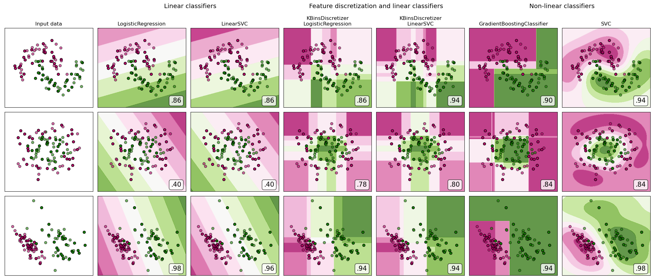
在合成分类数据集上进行特征离散化的演示。特征离散化将每个特征分解为一组bin,此处的宽度均匀分布。然后将离散值进行一次热编码,并提供给线性分类器。即使分类器是线性的,此预处理也可以实现非线性行为。
在此示例中,前两行代表线性不可分离的数据集(月亮和同心圆),而第三行则近似线性可分离。在两个线性不可分离的数据集上,特征离散化大大提高了线性分类器的性能。在线性可分离数据集上,特征离散化会降低线性分类器的性能。还显示了两个非线性分类器以进行比较。
此示例应以一粒盐为准,因为传达的直觉不一定会延续到实际数据集中。特别是在高维空间中,可以更轻松地线性分离数据。此外,使用特征离散化和一键编码增加了特征数量,当样本数量少时,容易导致过度拟合。
这些图以纯色显示训练点,测试点是半透明的。右下方显示了测试集上的分类准确性。
# 源代码: Tom Dupré la Tour
# 改编自Gaël Varoquaux和Andreas Müller的plot_classifier_comparison
#
# 执照: BSD 3 clause

import numpy as np
import matplotlib.pyplot as plt
from matplotlib.colors import ListedColormap
from sklearn.model_selection import train_test_split
from sklearn.preprocessing import StandardScaler
from sklearn.datasets import make_moons, make_circles, make_classification
from sklearn.linear_model import LogisticRegression
from sklearn.model_selection import GridSearchCV
from sklearn.pipeline import make_pipeline
from sklearn.preprocessing import KBinsDiscretizer
from sklearn.svm import SVC, LinearSVC
from sklearn.ensemble import GradientBoostingClassifier
from sklearn.utils._testing import ignore_warnings
from sklearn.exceptions import ConvergenceWarning

print(__doc__)

h = .02  # 设置网格的补不长


def get_name(estimator):
    name = estimator.__class__.__name__
    if name == 'Pipeline':
        name = [get_name(est[1]) for est in estimator.steps]
        name = ' + '.join(name)
    return name


# (estimator,param_grid)的列表,其中在GridSearchCV中使用param_grid
classifiers = [
    (LogisticRegression(random_state=0), {
        'C': np.logspace(-2, 7, 10)
    }),
    (LinearSVC(random_state=0), {
        'C': np.logspace(-2, 7, 10)
    }),
    (make_pipeline(
        KBinsDiscretizer(encode='onehot'),
        LogisticRegression(random_state=0)), {
            'kbinsdiscretizer__n_bins': np.arange(2, 10),
            'logisticregression__C': np.logspace(-2, 7, 10),
        }),
    (make_pipeline(
        KBinsDiscretizer(encode='onehot'), LinearSVC(random_state=0)), {
            'kbinsdiscretizer__n_bins': np.arange(2, 10),
            'linearsvc__C': np.logspace(-2, 7, 10),
        }),
    (GradientBoostingClassifier(n_estimators=50, random_state=0), {
        'learning_rate': np.logspace(-4, 0, 10)
    }),
    (SVC(random_state=0), {
        'C': np.logspace(-2, 7, 10)
    }),
]

names = [get_name(e) for e, g in classifiers]

n_samples = 100
datasets = [
    make_moons(n_samples=n_samples, noise=0.2, random_state=0),
    make_circles(n_samples=n_samples, noise=0.2, factor=0.5, random_state=1),
    make_classification(n_samples=n_samples, n_features=2, n_redundant=0,
                        n_informative=2, random_state=2,
                        n_clusters_per_class=1)
]

fig, axes = plt.subplots(nrows=len(datasets), ncols=len(classifiers) + 1,
                         figsize=(21, 9))

cm = plt.cm.PiYG
cm_bright = ListedColormap(['#b30065', '#178000'])

# 在数据集上迭代
for ds_cnt, (X, y) in enumerate(datasets):
    print('\ndataset %d\n---------' % ds_cnt)

    # 预处理数据集,分为训练和测试部分
    X = StandardScaler().fit_transform(X)
    X_train, X_test, y_train, y_test = train_test_split(
        X, y, test_size=.5, random_state=42)

    # 为背景颜色创建网格
    x_min, x_max = X[:, 0].min() - .5, X[:, 0].max() + .5
    y_min, y_max = X[:, 1].min() - .5, X[:, 1].max() + .5
    xx, yy = np.meshgrid(
        np.arange(x_min, x_max, h), np.arange(y_min, y_max, h))

    # 首先绘制数据集
    ax = axes[ds_cnt, 0]
    if ds_cnt == 0:
        ax.set_title("Input data")
    # plot the training points
    ax.scatter(X_train[:, 0], X_train[:, 1], c=y_train, cmap=cm_bright,
               edgecolors='k')
    # and testing points
    ax.scatter(X_test[:, 0], X_test[:, 1], c=y_test, cmap=cm_bright, alpha=0.6,
               edgecolors='k')
    ax.set_xlim(xx.min(), xx.max())
    ax.set_ylim(yy.min(), yy.max())
    ax.set_xticks(())
    ax.set_yticks(())

    # 在分类器上迭代
    for est_idx, (name, (estimator, param_grid)) in \
            enumerate(zip(names, classifiers)):
        ax = axes[ds_cnt, est_idx + 1]

        clf = GridSearchCV(estimator=estimator, param_grid=param_grid)
        with ignore_warnings(category=ConvergenceWarning):
            clf.fit(X_train, y_train)
        score = clf.score(X_test, y_test)
        print('%s: %.2f' % (name, score))

        # 绘制决策边界。
        # 我们将为网格[x_min,x_max] * [y_min,y_max]中的每个点分配颜色。
        if hasattr(clf, "decision_function"):
            Z = clf.decision_function(np.c_[xx.ravel(), yy.ravel()])
        else:
            Z = clf.predict_proba(np.c_[xx.ravel(), yy.ravel()])[:, 1]

        # 将结果放入颜色图
        Z = Z.reshape(xx.shape)
        ax.contourf(xx, yy, Z, cmap=cm, alpha=.8)

        # 绘制训练点
        ax.scatter(X_train[:, 0], X_train[:, 1], c=y_train, cmap=cm_bright,
                   edgecolors='k')
        # 以及测试点
        ax.scatter(X_test[:, 0], X_test[:, 1], c=y_test, cmap=cm_bright,
                   edgecolors='k', alpha=0.6)
        ax.set_xlim(xx.min(), xx.max())
        ax.set_ylim(yy.min(), yy.max())
        ax.set_xticks(())
        ax.set_yticks(())

        if ds_cnt == 0:
            ax.set_title(name.replace(' + ', '\n'))
        ax.text(0.95, 0.06, ('%.2f' % score).lstrip('0'), size=15,
                bbox=dict(boxstyle='round', alpha=0.8, facecolor='white'),
                transform=ax.transAxes, horizontalalignment='right')


plt.tight_layout()

# 在图像上增加标题
plt.subplots_adjust(top=0.90)
suptitles = [
    'Linear classifiers',
    'Feature discretization and linear classifiers',
    'Non-linear classifiers',
]
for i, suptitle in zip([1, 3, 5], suptitles):
    ax = axes[0, i]
    ax.text(1.05, 1.25, suptitle, transform=ax.transAxes,
            horizontalalignment='center', size='x-large')
plt.show()
输出:
dataset 0
---------
LogisticRegression: 0.86
LinearSVC: 0.86
KBinsDiscretizer + LogisticRegression: 0.86
KBinsDiscretizer + LinearSVC: 0.92
GradientBoostingClassifier: 0.90
SVC: 0.94

dataset 1
---------
LogisticRegression: 0.40
LinearSVC: 0.40
KBinsDiscretizer + LogisticRegression: 0.88
KBinsDiscretizer + LinearSVC: 0.86
GradientBoostingClassifier: 0.80
SVC: 0.84

dataset 2
---------
LogisticRegression: 0.98
LinearSVC: 0.98
KBinsDiscretizer + LogisticRegression: 0.94
KBinsDiscretizer + LinearSVC: 0.94
GradientBoostingClassifier: 0.88
SVC: 0.98
脚本的总运行时间:(0分钟25.699秒)

