将数据映射到正态分布¶

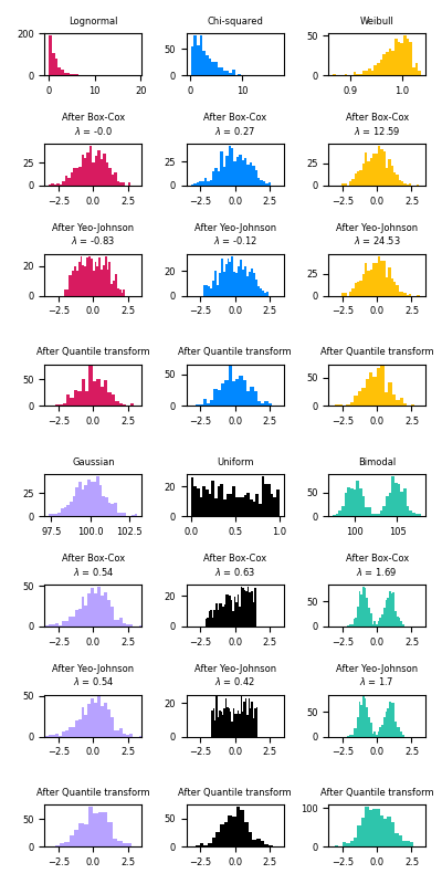
本示例演示通过PowerTransformer使用Box-Cox和Yeo-Johnson变换将数据从各种分布映射到正态分布。

幂变换可用作在建模中需要均等和正态的问题的变换。以下是适用于六个不同概率分布的Box-Cox和Yeo-Johnwon的示例：对数正态，卡方，威布尔，高斯，均匀和双峰。

请注意，当应用于某些数据集时，转换成功地将数据映射到正态分布，但对其他数据集无效。这突出了在转换之前和之后可视化数据的重要性。

还要注意，即使Box-Cox在对数正态分布和卡方分布方面的表现似乎比Yeo-Johnson好，但请记住Box-Cox不支持负值输入。

为了进行比较，我们还添加了QuantileTransformer的输出。只要有足够的训练样本（数千个），它就可以将任意分布强加给高斯。因为它是非参数方法，所以比参数方法（Box-Cox和Yeo-Johnson）更难解释。

在“小型”数据集（少于几百个点）上，分位数转换器容易过拟合。然后建议使用功率变换。

# 作者: Eric Chang <ericchang2017@u.northwestern.edu>
#         Nicolas Hug <contact@nicolas-hug.com>
# 执照: BSD 3 clause

import numpy as np
import matplotlib.pyplot as plt

from sklearn.preprocessing import PowerTransformer
from sklearn.preprocessing import QuantileTransformer
from sklearn.model_selection import train_test_split

print(__doc__)


N_SAMPLES = 1000
FONT_SIZE = 6
BINS = 30


rng = np.random.RandomState(304)
bc = PowerTransformer(method='box-cox')
yj = PowerTransformer(method='yeo-johnson')
# n_quantiles设置为训练集大小，而不是默认值，以避免此示例引发警告
qt = QuantileTransformer(n_quantiles=500, output_distribution='normal',
                         random_state=rng)
size = (N_SAMPLES, 1)


# 对数正态分布
X_lognormal = rng.lognormal(size=size)

# 卡方分布
df = 3
X_chisq = rng.chisquare(df=df, size=size)

# 威布尔分布
a = 50
X_weibull = rng.weibull(a=a, size=size)

# 高斯分布
loc = 100
X_gaussian = rng.normal(loc=loc, size=size)

# 均匀分布
X_uniform = rng.uniform(low=0, high=1, size=size)

# 双峰分布
loc_a, loc_b = 100, 105
X_a, X_b = rng.normal(loc=loc_a, size=size), rng.normal(loc=loc_b, size=size)
X_bimodal = np.concatenate([X_a, X_b], axis=0)


# 绘制图像
distributions = [
    ('Lognormal', X_lognormal),
    ('Chi-squared', X_chisq),
    ('Weibull', X_weibull),
    ('Gaussian', X_gaussian),
    ('Uniform', X_uniform),
    ('Bimodal', X_bimodal)
]

colors = ['#D81B60', '#0188FF', '#FFC107',
          '#B7A2FF', '#000000', '#2EC5AC']

fig, axes = plt.subplots(nrows=8, ncols=3, figsize=plt.figaspect(2))
axes = axes.flatten()
axes_idxs = [(0, 3, 6, 9), (1, 4, 7, 10), (2, 5, 8, 11), (12, 15, 18, 21),
             (13, 16, 19, 22), (14, 17, 20, 23)]
axes_list = [(axes[i], axes[j], axes[k], axes[l])
             for (i, j, k, l) in axes_idxs]


for distribution, color, axes in zip(distributions, colors, axes_list):
    name, X = distribution
    X_train, X_test = train_test_split(X, test_size=.5)

    # 执行幂变换和分位数变换
    X_trans_bc = bc.fit(X_train).transform(X_test)
    lmbda_bc = round(bc.lambdas_[0], 2)
    X_trans_yj = yj.fit(X_train).transform(X_test)
    lmbda_yj = round(yj.lambdas_[0], 2)
    X_trans_qt = qt.fit(X_train).transform(X_test)

    ax_original, ax_bc, ax_yj, ax_qt = axes

    ax_original.hist(X_train, color=color, bins=BINS)
    ax_original.set_title(name, fontsize=FONT_SIZE)
    ax_original.tick_params(axis='both', which='major', labelsize=FONT_SIZE)

    for ax, X_trans, meth_name, lmbda in zip(
            (ax_bc, ax_yj, ax_qt),
            (X_trans_bc, X_trans_yj, X_trans_qt),
            ('Box-Cox', 'Yeo-Johnson', 'Quantile transform'),
            (lmbda_bc, lmbda_yj, None)):
        ax.hist(X_trans, color=color, bins=BINS)
        title = 'After {}'.format(meth_name)
        if lmbda is not None:
            title += r'\n$\lambda$ = {}'.format(lmbda)
        ax.set_title(title, fontsize=FONT_SIZE)
        ax.tick_params(axis='both', which='major', labelsize=FONT_SIZE)
        ax.set_xlim([-3.5, 3.5])


plt.tight_layout()
plt.show()

输出：

脚本的总运行时间：（0分钟2.021秒）