管道：链接PCA和逻辑回归¶

PCA可进行无监督的降维，而使用逻辑回归进行预测。

我们使用GridSearchCV设置PCA的维度。

print(__doc__)


# 源代码: Gaël Varoquaux
# 由Jaques Grobler修改为文档
# 执照: BSD 3 clause


import numpy as np
import matplotlib.pyplot as plt
import pandas as pd

from sklearn import datasets
from sklearn.decomposition import PCA
from sklearn.linear_model import LogisticRegression
from sklearn.pipeline import Pipeline
from sklearn.model_selection import GridSearchCV


# 定义管道以搜索PCA截断和分类器正则化的最佳组合。
pca = PCA()
# 将公差设置为较大的值可以使示例更快
logistic = LogisticRegression(max_iter=10000, tol=0.1)
pipe = Pipeline(steps=[('pca', pca), ('logistic', logistic)])

X_digits, y_digits = datasets.load_digits(return_X_y=True)

# 可以使用__分隔的参数名称来设置管道的参数：
param_grid = {
    'pca__n_components': [5, 15, 30, 45, 64],
    'logistic__C': np.logspace(-4, 4, 4),
}
search = GridSearchCV(pipe, param_grid, n_jobs=-1)
search.fit(X_digits, y_digits)
print("Best parameter (CV score=%0.3f):" % search.best_score_)
print(search.best_params_)

# 绘制PCA频谱：
pca.fit(X_digits)

fig, (ax0, ax1) = plt.subplots(nrows=2, sharex=True, figsize=(6, 6))
ax0.plot(np.arange(1, pca.n_components_ + 1),
         pca.explained_variance_ratio_, '+', linewidth=2)
ax0.set_ylabel('PCA explained variance ratio')

ax0.axvline(search.best_estimator_.named_steps['pca'].n_components,
            linestyle=':', label='n_components chosen')
ax0.legend(prop=dict(size=12))

# 对于每种数量的组件，找到最佳的分类器结果
results = pd.DataFrame(search.cv_results_)
components_col = 'param_pca__n_components'
best_clfs = results.groupby(components_col).apply(
    lambda g: g.nlargest(1, 'mean_test_score'))

best_clfs.plot(x=components_col, y='mean_test_score', yerr='std_test_score',
               legend=False, ax=ax1)
ax1.set_ylabel('Classification accuracy (val)')
ax1.set_xlabel('n_components')

plt.xlim(-1, 70)

plt.tight_layout()
plt.show()

输出：

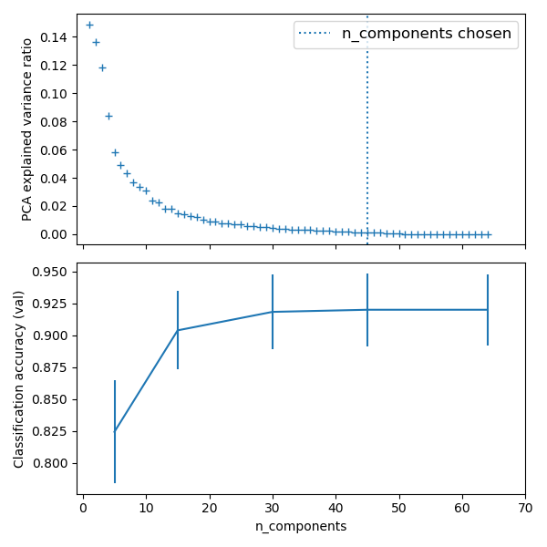
Best parameter (CV score=0.920):
{'logistic__C': 0.046415888336127774, 'pca__n_components': 45}

脚本的总运行时间：（0分钟15.214秒）