

嵌套与非嵌套交叉验证
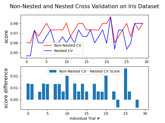
本案例在鸢尾花数据集的分类器上比较了非嵌套和嵌套的交叉验证策略。嵌套交叉验证(CV)通常用于训练还需要优化超参数的模型。嵌套交叉验证估计基础模型及其(超)参数搜索的泛化误差。选择最大化非嵌套交叉验证结果的参数会使模型偏向数据集,从而产生过于乐观的得分。
没有嵌套CV的模型选择使用相同的数据来调整模型参数并评估模型性能。因此,信息可能会“渗入”模型并过拟合数据。这种影响的大小主要取决于数据集的大小和模型的稳定性。有关这些问题的分析,请参见Cawley and Talbot(引用1)。
为避免此问题,嵌套CV有效地使用了一系列训练/验证/测试集拆分。在内部循环(在此由GridSearchCV执行)中,通过将模型拟合到每个训练集来近似最大化分数,然后在验证集上选择(超)参数时直接将其最大化。在外部循环中(此处为cross_val_score),通过对几个数据集拆分中的测试集得分求平均值来估计泛化误差。
下面的示例使用带有非线性核的支持向量分类器,通过网格搜索构建具有优化超参数的模型。通过比较非嵌套和嵌套CV策略得分之间的差异,我们可以比较它们的效果。
同时查看:
引用:
输出:
Average difference of 0.007581 with std. dev. of 0.007833.
输入:
from sklearn.datasets import load_iris
from matplotlib import pyplot as plt
from sklearn.svm import SVC
from sklearn.model_selection import GridSearchCV, cross_val_score, KFold
import numpy as np

print(__doc__)

# 随机试验次数
NUM_TRIALS = 30

# 导入数据集
iris = load_iris()
X_iris = iris.data
y_iris = iris.target

# 设置参数的可能值以优化
p_grid = {"C": [1, 10, 100],
          "gamma": [.01, .1]}

# 我们将使用带有“ rbf”内核的支持向量分类器
svm = SVC(kernel="rbf")

# 存储分数的数组
non_nested_scores = np.zeros(NUM_TRIALS)
nested_scores = np.zeros(NUM_TRIALS)

# 每次试用循环
for i in range(NUM_TRIALS):

    # 独立于数据集,为内部和外部循环选择交叉验证技术。
    # 例如“ GroupKFold”,“ LeaveOneOut”,“ LeaveOneGroupOut”等。
    inner_cv = KFold(n_splits=4, shuffle=True, random_state=i)
    outer_cv = KFold(n_splits=4, shuffle=True, random_state=i)

    # 非嵌套参数搜索和评分
    clf = GridSearchCV(estimator=svm, param_grid=p_grid, cv=inner_cv)
    clf.fit(X_iris, y_iris)
    non_nested_scores[i] = clf.best_score_

    # 带有参数优化的嵌套简历
    nested_score = cross_val_score(clf, X=X_iris, y=y_iris, cv=outer_cv)
    nested_scores[i] = nested_score.mean()

score_difference = non_nested_scores - nested_scores

print("Average difference of {:6f} with std. dev. of {:6f}."
      .format(score_difference.mean(), score_difference.std()))

# 嵌套和非嵌套CV在每个试验中的得分
plt.figure()
plt.subplot(211)
non_nested_scores_line, = plt.plot(non_nested_scores, color='r')
nested_line, = plt.plot(nested_scores, color='b')
plt.ylabel("score", fontsize="14")
plt.legend([non_nested_scores_line, nested_line],
           ["Non-Nested CV", "Nested CV"],
           bbox_to_anchor=(0, .4, .5, 0))
plt.title("Non-Nested and Nested Cross Validation on Iris Dataset",
          x=.5, y=1.1, fontsize="15")

# Plot bar chart of the difference.
plt.subplot(212)
difference_plot = plt.bar(range(NUM_TRIALS), score_difference)
plt.xlabel("Individual Trial #")
plt.legend([difference_plot],
           ["Non-Nested CV - Nested CV Score"],
           bbox_to_anchor=(0, 1, .8, 0))
plt.ylabel("score difference", fontsize="14")

plt.show()
脚本的总运行时间:(0分钟6.053秒)

