使用IterativeImputer的变体估算缺失值¶

sklearn.impute.IterativeImputer类非常灵活：它可以与各种估算器一起使用以进行循环回归，将每个变量依次作为输出。

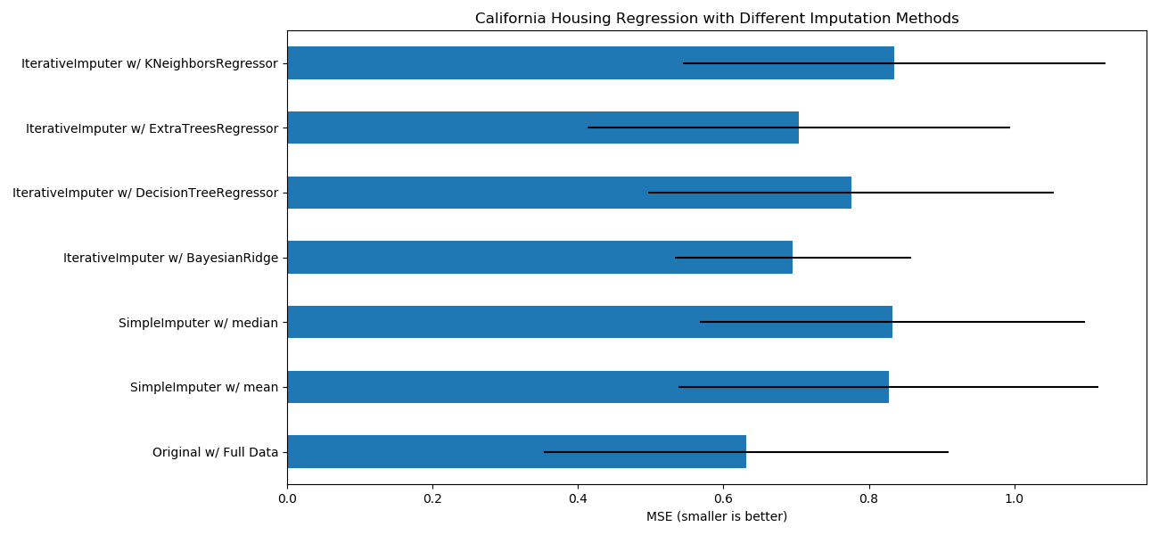
在此示例中，我们将一些估计器与sklearn.impute.IterativeImputer进行了比较，以估计缺失的特征：

• BayesianRidge：贝叶斯领回归，一种正则线性回归

• DecisionTreeRegressor：决策树回归，非线性回归

• ExtraTreesRegressor：额外树回归，类似于R中的missForest

• KNeighborsRegressor：K近邻回归，与其他KNN插补方法相当

特别令人感兴趣的是sklearn.impute.IterativeImputer用以模仿missForest（R的流行插补包）行为的功能。在此示例中，我们选择使用sklearn.ensemble.ExtraTreesRegressor而不是sklearn.ensemble.RandomForestRegressor（如missForest），因为它提高了速度。

请注意，sklearn.neighbors.KNeighborsRegressor与KNN插补不同，后者通过使用考虑缺失值而不是插补的距离度量从缺失值的样本中学习。

目标是比较不同的估算器，以查看在加利福尼亚住房数据集中使用sklearn.linear_model.BayesianRidge估算器时，哪一个最适合sklearn.impute.IterativeImputer，并且从各行中随机删除一个值。

对于这种特殊的缺失值模式，我们看到sklearn.ensemble.ExtraTreesRegressor和sklearn.linear_model.BayesianRidge提供了最佳结果。

输入：

print(__doc__)

import numpy as np
import matplotlib.pyplot as plt
import pandas as pd

# 要使用此实验特性，我们需要明确引入以下包和库：
from sklearn.experimental import enable_iterative_imputer  # noqa
from sklearn.datasets import fetch_california_housing
from sklearn.impute import SimpleImputer
from sklearn.impute import IterativeImputer
from sklearn.linear_model import BayesianRidge
from sklearn.tree import DecisionTreeRegressor
from sklearn.ensemble import ExtraTreesRegressor
from sklearn.neighbors import KNeighborsRegressor
from sklearn.pipeline import make_pipeline
from sklearn.model_selection import cross_val_score

N_SPLITS = 5

rng = np.random.RandomState(0)

X_full, y_full = fetch_california_housing(return_X_y=True)
# 就示例而言，大约2k个样本就足够了。
# 删除以下两行，能够使运行速度因不同的错误条而放慢。
X_full = X_full[::10]
y_full = y_full[::10]
n_samples, n_features = X_full.shape

# 估计整个数据集的分数，没有缺失值
br_estimator = BayesianRidge()
score_full_data = pd.DataFrame(
    cross_val_score(
        br_estimator, X_full, y_full, scoring='neg_mean_squared_error',
        cv=N_SPLITS
    ),
    columns=['Full Data']
)

# 每行添加一个缺失值
X_missing = X_full.copy()
y_missing = y_full
missing_samples = np.arange(n_samples)
missing_features = rng.choice(n_features, n_samples, replace=True)
X_missing[missing_samples, missing_features] = np.nan

# 估算插补后的得分（均值和中位数策略）
score_simple_imputer = pd.DataFrame()
for strategy in ('mean', 'median'):
    estimator = make_pipeline(
        SimpleImputer(missing_values=np.nan, strategy=strategy),
        br_estimator
    )
    score_simple_imputer[strategy] = cross_val_score(
        estimator, X_missing, y_missing, scoring='neg_mean_squared_error',
        cv=N_SPLITS
    )

# 在用不同的估计量迭代插补缺失值之后估计分数
estimators = [
    BayesianRidge(),
    DecisionTreeRegressor(max_features='sqrt', random_state=0),
    ExtraTreesRegressor(n_estimators=10, random_state=0),
    KNeighborsRegressor(n_neighbors=15)
]
score_iterative_imputer = pd.DataFrame()
for impute_estimator in estimators:
    estimator = make_pipeline(
        IterativeImputer(random_state=0, estimator=impute_estimator),
        br_estimator
    )
    score_iterative_imputer[impute_estimator.__class__.__name__] = \
        cross_val_score(
            estimator, X_missing, y_missing, scoring='neg_mean_squared_error',
            cv=N_SPLITS
        )

scores = pd.concat(
    [score_full_data, score_simple_imputer, score_iterative_imputer],
    keys=['Original', 'SimpleImputer', 'IterativeImputer'], axis=1
)

# 绘制加利福尼亚房屋价值数据集上的结果
fig, ax = plt.subplots(figsize=(13, 6))
means = -scores.mean()
errors = scores.std()
means.plot.barh(xerr=errors, ax=ax)
ax.set_title('California Housing Regression with Different Imputation Methods')
ax.set_xlabel('MSE (smaller is better)')
ax.set_yticks(np.arange(means.shape[0]))
ax.set_yticklabels([" w/ ".join(label) for label in means.index.tolist()])
plt.tight_layout(pad=1)
plt.show()

输出：

脚本的总运行时间：（0分钟26.278秒）。