

对“玩具数据集”进行异常检测,并比较异常检测算法
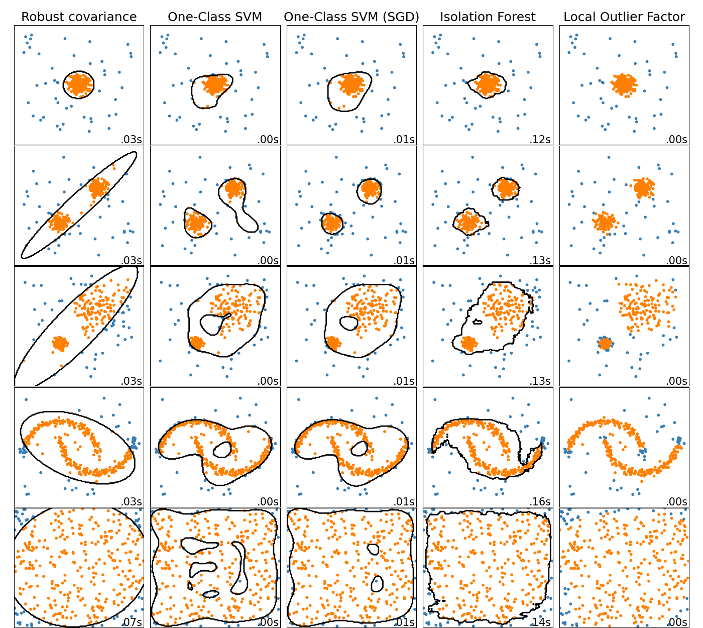
此示例显示了二维数据集上不同异常检测算法的特色。数据集包含一种或两种模式(高密度区域),以说明算法处理多模式数据的能力。
对于每个数据集,将生成15%的样本作为随机均匀噪声。该比例是为OneClassSVM的nu参数和其他异常值检测算法的污染参数提供的值。离群值和离群值之间的决策边界以黑色显示,但局部离群值因子(LOF)除外,因为当用于离群值检测时,它没有适用于新数据的预测方法。
已知sklearn.svm.OneClassSVM对异常值敏感,因此在异常值检测方面表现不佳。当训练集不受异常值污染时,此估算器最适合新颖性检测。也就是说,在高维中进行离群值检测,或者不对基础数据的分布进行任何假设,都是非常具有挑战性的,一类SVM在这些情况下可能会根据其超参数的值给出有用的结果。
sklearn.covariance.EllipticEnvelope假定数据为高斯并学习一个椭圆。因此,当数据不是单峰时,它会降级。但是请注意,此估计量对异常值具有鲁棒性。
对于多模式数据集,sklearn.ensemble.IsolationForest和sklearn.neighbors.LocalOutlierFactor的表现似乎相当不错。对于第三个数据集,显示了sklearn.neighbors.LocalOutlierFactor相对于其他估算器的优势,其中两个模式的密度不同。 LOF的局部方面解释了这一优势,这意味着它仅将一个样本的异常评分与其邻居的评分进行比较。
最后,对于最后一个数据集,很难说一个样本比另一个样本异常得多,因为它们均匀分布在超立方体中。除了sklearn.svm.OneClassSVM有点过拟合外,所有估算器都针对这种情况提供了不错的解决方案。在这种情况下,明智的做法是仔细观察样本的异常分数,因为好的估算者应该为所有样本分配相似的分数。
尽管这些示例给出了有关算法的一些直觉,但这种直觉可能不适用于非常高维的数据。
最后,请注意,此处已手动选择了模型的参数,但实际上需要对其进行调整。在没有标记数据的情况下,该问题是完全不受监督的,因此选择模型可能是一个挑战。
# 作者: Alexandre Gramfort <alexandre.gramfort@inria.fr>
#         Albert Thomas <albert.thomas@telecom-paristech.fr>
# 执照: BSD 3 clause

import time

import numpy as np
import matplotlib
import matplotlib.pyplot as plt

from sklearn import svm
from sklearn.datasets import make_moons, make_blobs
from sklearn.covariance import EllipticEnvelope
from sklearn.ensemble import IsolationForest
from sklearn.neighbors import LocalOutlierFactor

print(__doc__)

matplotlib.rcParams['contour.negative_linestyle'] = 'solid'

# 设置基本参数
n_samples = 300
outliers_fraction = 0.15
n_outliers = int(outliers_fraction * n_samples)
n_inliers = n_samples - n_outliers

# 定义需要比较的异常值/离群值检测方法
anomaly_algorithms = [
    ("Robust covariance", EllipticEnvelope(contamination=outliers_fraction)),
    ("One-Class SVM", svm.OneClassSVM(nu=outliers_fraction, kernel="rbf",
                                      gamma=0.1)),
    ("Isolation Forest", IsolationForest(contamination=outliers_fraction,
                                         random_state=42)),
    ("Local Outlier Factor", LocalOutlierFactor(
        n_neighbors=35, contamination=outliers_fraction))]

# 定义数据集
blobs_params = dict(random_state=0, n_samples=n_inliers, n_features=2)
datasets = [
    make_blobs(centers=[[0, 0], [0, 0]], cluster_std=0.5,
               **blobs_params)[0],
    make_blobs(centers=[[2, 2], [-2, -2]], cluster_std=[0.5, 0.5],
               **blobs_params)[0],
    make_blobs(centers=[[2, 2], [-2, -2]], cluster_std=[1.5, .3],
               **blobs_params)[0],
    4. * (make_moons(n_samples=n_samples, noise=.05, random_state=0)[0] -
          np.array([0.5, 0.25])),
    14. * (np.random.RandomState(42).rand(n_samples, 2) - 0.5)]

# 在给定的设定下,比较分类器
xx, yy = np.meshgrid(np.linspace(-7, 7, 150),
                     np.linspace(-7, 7, 150))

plt.figure(figsize=(len(anomaly_algorithms) * 2 + 3, 12.5))
plt.subplots_adjust(left=.02, right=.98, bottom=.001, top=.96, wspace=.05,
                    hspace=.01)

plot_num = 1
rng = np.random.RandomState(42)

for i_dataset, X in enumerate(datasets):
    # 增加离群值
    X = np.concatenate([X, rng.uniform(low=-6, high=6,
                       size=(n_outliers, 2))], axis=0)

    for name, algorithm in anomaly_algorithms:
        t0 = time.time()
        algorithm.fit(X)
        t1 = time.time()
        plt.subplot(len(datasets), len(anomaly_algorithms), plot_num)
        if i_dataset == 0:
            plt.title(name, size=18)

        # 拟合数据并标记出离群值
        if name == "Local Outlier Factor":
            y_pred = algorithm.fit_predict(X)
        else:
            y_pred = algorithm.fit(X).predict(X)

        # 绘制等高线以及点
        if name != "Local Outlier Factor":  # LOF不执行预测
            Z = algorithm.predict(np.c_[xx.ravel(), yy.ravel()])
            Z = Z.reshape(xx.shape)
            plt.contour(xx, yy, Z, levels=[0], linewidths=2, colors='black')

        colors = np.array(['#377eb8', '#ff7f00'])
        plt.scatter(X[:, 0], X[:, 1], s=10, color=colors[(y_pred + 1) // 2])

        plt.xlim(-7, 7)
        plt.ylim(-7, 7)
        plt.xticks(())
        plt.yticks(())
        plt.text(.99, .01, ('%.2fs' % (t1 - t0)).lstrip('0'),
                 transform=plt.gca().transAxes, size=15,
                 horizontalalignment='right')
        plot_num += 1

plt.show()
输出:
脚本的总运行时间:(0分钟7.474秒)

