

Johnson-Lindenstrauss绑定嵌入随机投影
Johnson-Lindenstrauss引理指出,任何高维数据集都可以随机投影到低维欧几里得空间中,同时控制成对距离的畸变。
print(__doc__)

import sys
from time import time
import numpy as np
import matplotlib
import matplotlib.pyplot as plt
from distutils.version import LooseVersion
from sklearn.random_projection import johnson_lindenstrauss_min_dim
from sklearn.random_projection import SparseRandomProjection
from sklearn.datasets import fetch_20newsgroups_vectorized
from sklearn.datasets import load_digits
from sklearn.metrics.pairwise import euclidean_distances

# 不推荐使用“规范”选项,更赞成使用直方图中的“密度”
if LooseVersion(matplotlib.__version__) >= '2.1':
    density_param = {'density': True}
else:
    density_param = {'normed': True}
理论界限
随机投影p引入的失真是由以下事实所断定的:p正在以很高的概率定义eps嵌入,其定义如下:
其中u和v是从形状[n_samples,n_features]形状的数据集中获取的任何行,而p是形状为[n_components,n_features]的随机高斯N(0,1)矩阵(或稀疏的Achlioptas矩阵)的投影。
保证eps嵌入的最小组件数由下式给出:
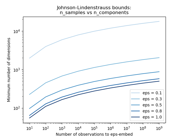
第一个图显示,随着样本数量n_samples的增加,最小维度n_components的数量对数地增加,以保证eps嵌入。
# 允许变形的范围
eps_range = np.linspace(0.1, 0.99, 5)
colors = plt.cm.Blues(np.linspace(0.3, 1.0, len(eps_range)))

# 嵌入的样本数(观测值)范围
n_samples_range = np.logspace(1, 9, 9)

plt.figure()
for eps, color in zip(eps_range, colors):
    min_n_components = johnson_lindenstrauss_min_dim(n_samples_range, eps=eps)
    plt.loglog(n_samples_range, min_n_components, color=color)

plt.legend(["eps = %0.1f" % eps for eps in eps_range], loc="lower right")
plt.xlabel("Number of observations to eps-embed")
plt.ylabel("Minimum number of dimensions")
plt.title("Johnson-Lindenstrauss bounds:\nn_samples vs n_components")
plt.show()
输出:
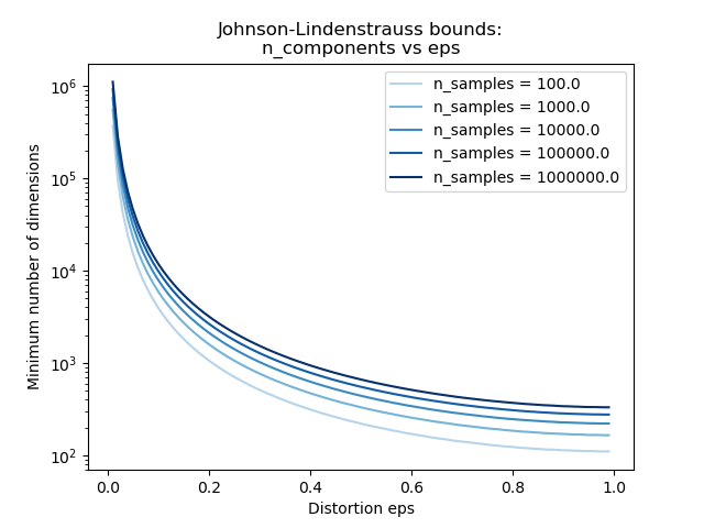
第二个图显示,对于给定数量的样本n_samples,允许失真eps的增加允许大幅减少最小维数n_components:
# 允许变形的范围
eps_range = np.linspace(0.01, 0.99, 100)

# 嵌入的样本数(观测值)范围
n_samples_range = np.logspace(2, 6, 5)
colors = plt.cm.Blues(np.linspace(0.3, 1.0, len(n_samples_range)))

plt.figure()
for n_samples, color in zip(n_samples_range, colors):
    min_n_components = johnson_lindenstrauss_min_dim(n_samples, eps=eps_range)
    plt.semilogy(eps_range, min_n_components, color=color)

plt.legend(["n_samples = %d" % n for n in n_samples_range], loc="upper right")
plt.xlabel("Distortion eps")
plt.ylabel("Minimum number of dimensions")
plt.title("Johnson-Lindenstrauss bounds:\nn_components vs eps")
plt.show()
输出:
实证验证
我们在20个新闻组文本文档(TF-IDF词频)数据集或数字数据集上验证上述界限:
对于20个新闻组数据集,使用稀疏随机矩阵将总共500个具有100k要素的文档投影到较小的欧几里得空间,并为目标n_components维数提供不同的值。
对于数字数据集,用于500个手写数字图片的一些8x8灰度像素数据被随机投影到空间,用于各种较大数量的维n_component。
默认数据集是20个新闻组数据集。 要在digits数据集上运行示例,请将--use-digits-dataset命令行参数传递给此脚本。
if '--use-digits-dataset' in sys.argv:
    data = load_digits().data[:500]
else:
    data = fetch_20newsgroups_vectorized().data[:500]
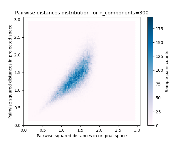
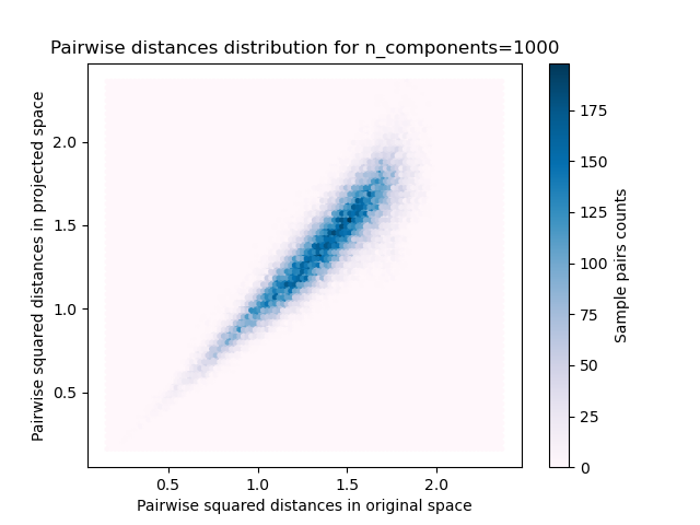
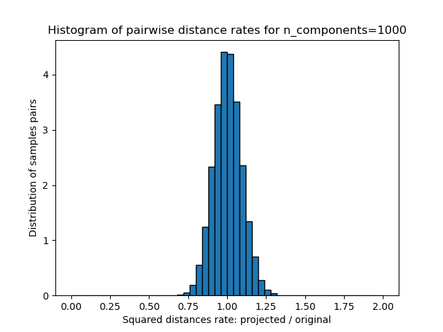
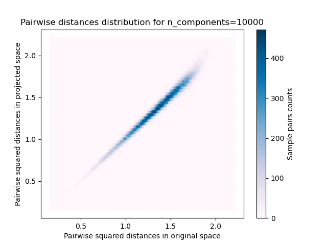
对于n_components的每个值,我们绘制:
原始和投影空间中成对距离的样本对的二维分布分别为x和y轴。
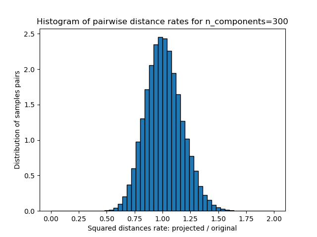
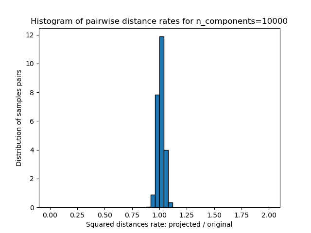
这些距离的比例的一维直方图(投影/原始)。
n_samples, n_features = data.shape
print("Embedding %d samples with dim %d using various random projections"
      % (n_samples, n_features))

n_components_range = np.array([300, 1000, 10000])
dists = euclidean_distances(data, squared=True).ravel()

# 仅选择不相同的样本对
nonzero = dists != 0
dists = dists[nonzero]

for n_components in n_components_range:
    t0 = time()
    rp = SparseRandomProjection(n_components=n_components)
    projected_data = rp.fit_transform(data)
    print("Projected %d samples from %d to %d in %0.3fs"
          % (n_samples, n_features, n_components, time() - t0))
    if hasattr(rp, 'components_'):
        n_bytes = rp.components_.data.nbytes
        n_bytes += rp.components_.indices.nbytes
        print("Random matrix with size: %0.3fMB" % (n_bytes / 1e6))

    projected_dists = euclidean_distances(
        projected_data, squared=True).ravel()[nonzero]

    plt.figure()
    min_dist = min(projected_dists.min(), dists.min())
    max_dist = max(projected_dists.max(), dists.max())
    plt.hexbin(dists, projected_dists, gridsize=100, cmap=plt.cm.PuBu,
               extent=[min_dist, max_dist, min_dist, max_dist])
    plt.xlabel("Pairwise squared distances in original space")
    plt.ylabel("Pairwise squared distances in projected space")
    plt.title("Pairwise distances distribution for n_components=%d" %
              n_components)
    cb = plt.colorbar()
    cb.set_label('Sample pairs counts')

    rates = projected_dists / dists
    print("Mean distances rate: %0.2f (%0.2f)"
          % (np.mean(rates), np.std(rates)))

    plt.figure()
    plt.hist(rates, bins=50, range=(0., 2.), edgecolor='k', **density_param)
    plt.xlabel("Squared distances rate: projected / original")
    plt.ylabel("Distribution of samples pairs")
    plt.title("Histogram of pairwise distance rates for n_components=%d" %
              n_components)

 # 待完成:计算eps的期望值并将其添加到上一个图
    # 作为垂直线/区域

plt.show()
输出:
Embedding 500 samples with dim 130107 using various random projections
Projected 500 samples from 130107 to 300 in 0.969s
Random matrix with size: 1.303MB
Mean distances rate: 1.01 (0.16)
Projected 500 samples from 130107 to 1000 in 3.381s
Random matrix with size: 4.325MB
Mean distances rate: 1.04 (0.11)
Projected 500 samples from 130107 to 10000 in 33.519s
Random matrix with size: 43.285MB
Mean distances rate: 0.99 (0.03)
我们可以看到,对于n_component的低值,分布较宽,具有许多扭曲对和偏斜的分布(由于左侧的零比率的硬性限制,因为距离始终为正),而对于n_component的较大值,则可以控制失真,并且通过随机投影可以很好地保持距离。
备注
根据JL引理,投影500个样本而没有太多失真将需要至少数千个维度,而与原始数据集的特征数量无关。
因此,对在输入空间中仅具有64个特征的数字数据集使用随机投影是没有意义的:在这种情况下,它不允许降维。
另一方面,在二十个新闻组中,维数可以从56436降低到10000,同时合理地保持成对的距离。
脚本的总运行时间:(0分钟43.639秒)

