

LASSO模型选择:交叉验证/AIC/BIC
利用Akaike信息准则(AIC)、Bayes信息准则(BIC)和交叉验证,选择Lasso估计器正则化参数alpha的最优值。
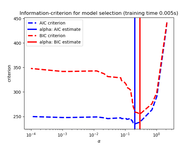
用LassoLarsIC得到的结果是基于AIC/BIC准则的。
基于信息准则的模型选择是非常快速的,但它依赖于适当的自由度估计,对大样本(渐近结果)进行推导,并假定模型是正确的,即数据实际上是由该模型生成的。当问题条件不好时(特征多于样本),它们也会崩溃。
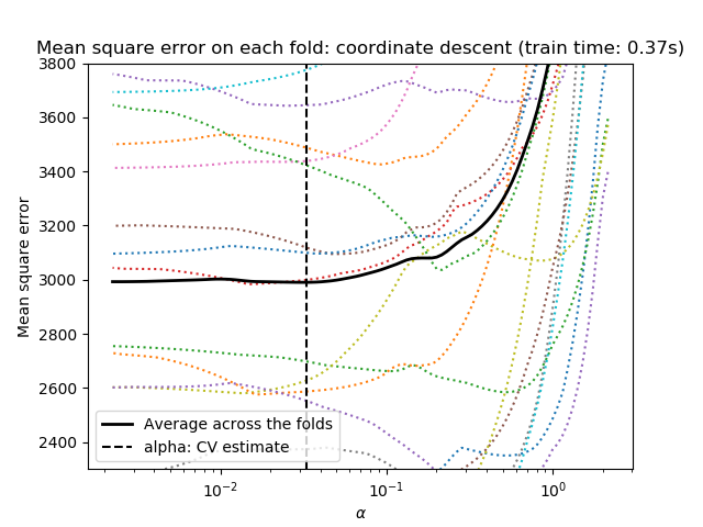
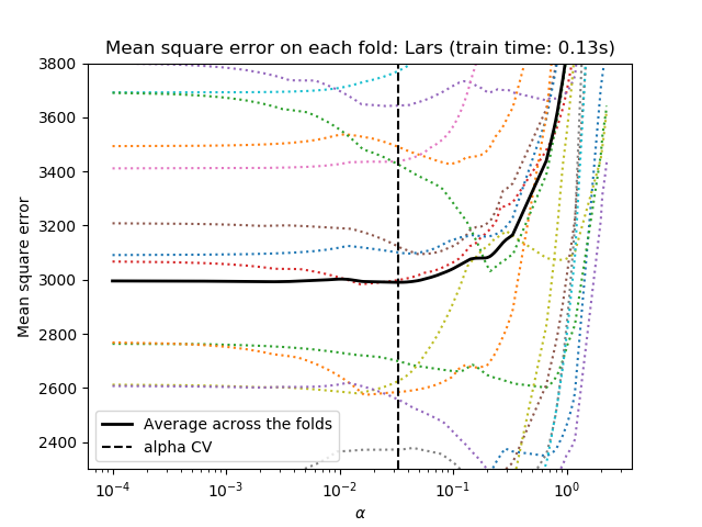
我们都使用20折交叉验证去计算2种算法计算Lasso路径:坐标下降(由LassoCV类实现)和LAS(最小角度回归)(由LassoLarsCV类实现)。这两种算法给出的结果大致相同。它们在执行速度和数值误差来源方面存在差异。的2种算法计算拉索路径:坐标下降(由LassoCV类实现)和LAS(最小角度回归)(由LassoLarsCV类实现)。这两种算法给出的结果大致相同。它们在执行速度和数值误差来源方面存在差异。
LARs只为路径中的每个扭结计算路径解决方案。因此,当只有少数几个扭结时,它是非常有效的,如果没有几个特征或样本,就会出现这种情况。此外,它还可以在不设置任何元参数的情况下计算完整路径。相反,坐标下降计算预先指定的网格上的路径点(这里我们使用默认值)。因此,如果网格点的数目小于路径中的扭结数,则效率更高。如果特征的数量非常多,并且有足够的样本来选择大量,那么这样的策略可能会很有趣。在数值误差方面,对于高度相关的变量,Lars会积累更多的误差,而坐标下降算法只会对网格上的路径进行采样。
注意,alpha的最优值在每一次折叠时是如何变化的。这说明了为什么在试图评估通过交叉验证选择参数的方法的性能时,嵌套交叉验证是必要的:对于未见数据,这种参数选择可能不是最优的。
Computing regularization path using the coordinate descent lasso...
Computing regularization path using the Lars lasso...
print(__doc__)

# Author: Olivier Grisel, Gael Varoquaux, Alexandre Gramfort
# License: BSD 3 clause

import time

import numpy as np
import matplotlib.pyplot as plt

from sklearn.linear_model import LassoCV, LassoLarsCV, LassoLarsIC
from sklearn import datasets

# This is to avoid division by zero while doing np.log10
EPSILON = 1e-4

X, y = datasets.load_diabetes(return_X_y=True)

rng = np.random.RandomState(42)
X = np.c_[X, rng.randn(X.shape[0], 14)]  # add some bad features

# normalize data as done by Lars to allow for comparison
X /= np.sqrt(np.sum(X ** 2, axis=0))

# #############################################################################
# LassoLarsIC: least angle regression with BIC/AIC criterion

model_bic = LassoLarsIC(criterion='bic')
t1 = time.time()
model_bic.fit(X, y)
t_bic = time.time() - t1
alpha_bic_ = model_bic.alpha_

model_aic = LassoLarsIC(criterion='aic')
model_aic.fit(X, y)
alpha_aic_ = model_aic.alpha_


def plot_ic_criterion(model, name, color):
    criterion_ = model.criterion_
    plt.semilogx(model.alphas_ + EPSILON, criterion_, '--', color=color,
                 linewidth=3, label='%s criterion' % name)
    plt.axvline(model.alpha_ + EPSILON, color=color, linewidth=3,
                label='alpha: %s estimate' % name)
    plt.xlabel(r'$\alpha$')
    plt.ylabel('criterion')


plt.figure()
plot_ic_criterion(model_aic, 'AIC', 'b')
plot_ic_criterion(model_bic, 'BIC', 'r')
plt.legend()
plt.title('Information-criterion for model selection (training time %.3fs)'
          % t_bic)

# #############################################################################
# LassoCV: coordinate descent

# Compute paths
print("Computing regularization path using the coordinate descent lasso...")
t1 = time.time()
model = LassoCV(cv=20).fit(X, y)
t_lasso_cv = time.time() - t1

# Display results
plt.figure()
ymin, ymax = 2300, 3800
plt.semilogx(model.alphas_ + EPSILON, model.mse_path_, ':')
plt.plot(model.alphas_ + EPSILON, model.mse_path_.mean(axis=-1), 'k',
         label='Average across the folds', linewidth=2)
plt.axvline(model.alpha_ + EPSILON, linestyle='--', color='k',
            label='alpha: CV estimate')

plt.legend()

plt.xlabel(r'$\alpha$')
plt.ylabel('Mean square error')
plt.title('Mean square error on each fold: coordinate descent '
          '(train time: %.2fs)' % t_lasso_cv)
plt.axis('tight')
plt.ylim(ymin, ymax)

# #############################################################################
# LassoLarsCV: least angle regression

# Compute paths
print("Computing regularization path using the Lars lasso...")
t1 = time.time()
model = LassoLarsCV(cv=20).fit(X, y)
t_lasso_lars_cv = time.time() - t1

# Display results
plt.figure()
plt.semilogx(model.cv_alphas_ + EPSILON, model.mse_path_, ':')
plt.semilogx(model.cv_alphas_ + EPSILON, model.mse_path_.mean(axis=-1), 'k',
             label='Average across the folds', linewidth=2)
plt.axvline(model.alpha_, linestyle='--', color='k',
            label='alpha CV')
plt.legend()

plt.xlabel(r'$\alpha$')
plt.ylabel('Mean square error')
plt.title('Mean square error on each fold: Lars (train time: %.2fs)'
          % t_lasso_lars_cv)
plt.axis('tight')
plt.ylim(ymin, ymax)

plt.show()
脚本的总运行时间:(0分1.212秒)

