

自动相关性确定回归(ARD)
拟合回归模型与贝叶斯岭回归。
有关回归者的更多信息,请参见贝叶斯岭回归。
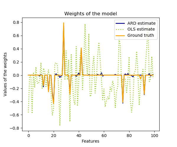
与普通最小二乘估计相比,系数权值略有移向零,从而使其稳定。
估计的权重的直方图是非常尖顶的,因为在权重上隐含了稀疏性的先验。
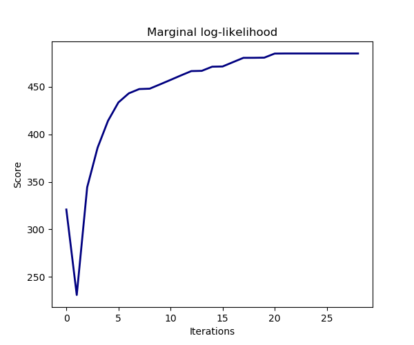
模型的估计是通过迭代最大化观测的边际对数似然来实现的。
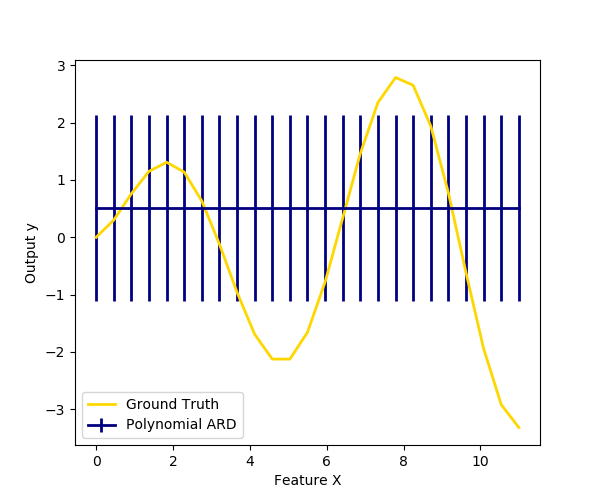
我们还用多项式特征扩展法绘制了一维回归ARD的预测和不确定性图。请注意,在右边的图中不确定性开始上升。这是因为这些测试样本超出了训练样本的范围。

print(__doc__)

import numpy as np
import matplotlib.pyplot as plt
from scipy import stats

from sklearn.linear_model import ARDRegression, LinearRegression

# #############################################################################
# Generating simulated data with Gaussian weights

# Parameters of the example
np.random.seed(0)
n_samples, n_features = 100, 100
# Create Gaussian data
X = np.random.randn(n_samples, n_features)
# Create weights with a precision lambda_ of 4.
lambda_ = 4.
w = np.zeros(n_features)
# Only keep 10 weights of interest
relevant_features = np.random.randint(0, n_features, 10)
for i in relevant_features:
    w[i] = stats.norm.rvs(loc=0, scale=1. / np.sqrt(lambda_))
# Create noise with a precision alpha of 50.
alpha_ = 50.
noise = stats.norm.rvs(loc=0, scale=1. / np.sqrt(alpha_), size=n_samples)
# Create the target
y = np.dot(X, w) + noise

# #############################################################################
# Fit the ARD Regression
clf = ARDRegression(compute_score=True)
clf.fit(X, y)

ols = LinearRegression()
ols.fit(X, y)

# #############################################################################
# Plot the true weights, the estimated weights, the histogram of the
# weights, and predictions with standard deviations
plt.figure(figsize=(6, 5))
plt.title("Weights of the model")
plt.plot(clf.coef_, color='darkblue', linestyle='-', linewidth=2,
         label="ARD estimate")
plt.plot(ols.coef_, color='yellowgreen', linestyle=':', linewidth=2,
         label="OLS estimate")
plt.plot(w, color='orange', linestyle='-', linewidth=2, label="Ground truth")
plt.xlabel("Features")
plt.ylabel("Values of the weights")
plt.legend(loc=1)

plt.figure(figsize=(6, 5))
plt.title("Histogram of the weights")
plt.hist(clf.coef_, bins=n_features, color='navy', log=True)
plt.scatter(clf.coef_[relevant_features], np.full(len(relevant_features), 5.),
            color='gold', marker='o', label="Relevant features")
plt.ylabel("Features")
plt.xlabel("Values of the weights")
plt.legend(loc=1)

plt.figure(figsize=(6, 5))
plt.title("Marginal log-likelihood")
plt.plot(clf.scores_, color='navy', linewidth=2)
plt.ylabel("Score")
plt.xlabel("Iterations")


# Plotting some predictions for polynomial regression
def f(x, noise_amount):
    y = np.sqrt(x) * np.sin(x)
    noise = np.random.normal(0, 1, len(x))
    return y + noise_amount * noise


degree = 10
X = np.linspace(0, 10, 100)
y = f(X, noise_amount=1)
clf_poly = ARDRegression(threshold_lambda=1e5)
clf_poly.fit(np.vander(X, degree), y)

X_plot = np.linspace(0, 11, 25)
y_plot = f(X_plot, noise_amount=0)
y_mean, y_std = clf_poly.predict(np.vander(X_plot, degree), return_std=True)
plt.figure(figsize=(6, 5))
plt.errorbar(X_plot, y_mean, y_std, color='navy',
             label="Polynomial ARD", linewidth=2)
plt.plot(X_plot, y_plot, color='gold', linewidth=2,
         label="Ground Truth")
plt.ylabel("Output y")
plt.xlabel("Feature X")
plt.legend(loc="lower left")
plt.show()
脚本的总运行时间:(0分0.530秒)

