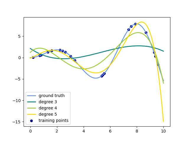
多项式插值¶

这个例子演示了如何用岭回归用n_degree多项式逼近一个函数。具体而言，从n_samples 1D点 出发，建立Vandermonde矩阵就足够了，它是n个样本 x n_degree+1，其形式如下：

[[1, x_1, x_1 ** 2, x_1 ** 3, …],
  [1, x_2, x_2 ** 2, x_2 ** 3, …], …] 

直观地说，这个矩阵可以解释为伪特征矩阵(提高到某种幂的点)。该矩阵类似于(但不同于)由多项式核导出的矩阵。

此示例显示，您可以使用线性模型进行非线性回归，使用pipeline添加非线性特性。核方法扩展了这一思想，可以诱导出非常高(甚至无限)维数的特征空间。

print(__doc__)

# Author: Mathieu Blondel
#         Jake Vanderplas
# License: BSD 3 clause

import numpy as np
import matplotlib.pyplot as plt

from sklearn.linear_model import Ridge
from sklearn.preprocessing import PolynomialFeatures
from sklearn.pipeline import make_pipeline


def f(x):
    """ function to approximate by polynomial interpolation"""
    return x * np.sin(x)


# generate points used to plot
x_plot = np.linspace(0, 10, 100)

# generate points and keep a subset of them
x = np.linspace(0, 10, 100)
rng = np.random.RandomState(0)
rng.shuffle(x)
x = np.sort(x[:20])
y = f(x)

# create matrix versions of these arrays
X = x[:, np.newaxis]
X_plot = x_plot[:, np.newaxis]

colors = ['teal', 'yellowgreen', 'gold']
lw = 2
plt.plot(x_plot, f(x_plot), color='cornflowerblue', linewidth=lw,
         label="ground truth")
plt.scatter(x, y, color='navy', s=30, marker='o', label="training points")

for count, degree in enumerate([3, 4, 5]):
    model = make_pipeline(PolynomialFeatures(degree), Ridge())
    model.fit(X, y)
    y_plot = model.predict(X_plot)
    plt.plot(x_plot, y_plot, color=colors[count], linewidth=lw,
             label="degree %d" % degree)

plt.legend(loc='lower left')

plt.show()

脚本的总运行时间：(0分0.091秒)

Download Python source code:plot_polynomial_interpolation.py

Download Jupyter notebook:plot_polynomial_interpolation.ipynb