

普通最小二乘与岭回归差异
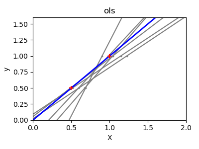
由于每个维度中的几个点以及线性回归所使用的直线尽可能地跟随这些点,观测数据上的噪声将导致第一幅图中所示的巨大差异。由于观测中产生的噪声,每条线的斜率对每个预测都会有很大的影响。
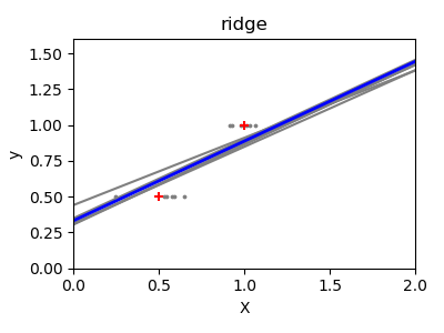
岭回归基本上是最小化最小二乘函数的惩罚版本。惩罚 shrinks了回归系数的值。与标准线性回归相比,尽管每个维的数据点较少,但预测的斜率要稳定得多,直线本身的方差也大大减小。
print(__doc__)


# Code source: Gaël Varoquaux
# Modified for documentation by Jaques Grobler
# License: BSD 3 clause


import numpy as np
import matplotlib.pyplot as plt

from sklearn import linear_model

X_train = np.c_[.5, 1].T
y_train = [.5, 1]
X_test = np.c_[0, 2].T

np.random.seed(0)

classifiers = dict(ols=linear_model.LinearRegression(),
                   ridge=linear_model.Ridge(alpha=.1))

for name, clf in classifiers.items():
    fig, ax = plt.subplots(figsize=(4, 3))

    for _ in range(6):
        this_X = .1 * np.random.normal(size=(2, 1)) + X_train
        clf.fit(this_X, y_train)

        ax.plot(X_test, clf.predict(X_test), color='gray')
        ax.scatter(this_X, y_train, s=3, c='gray', marker='o', zorder=10)

    clf.fit(X_train, y_train)
    ax.plot(X_test, clf.predict(X_test), linewidth=2, color='blue')
    ax.scatter(X_train, y_train, s=30, c='red', marker='+', zorder=10)

    ax.set_title(name)
    ax.set_xlim(0, 2)
    ax.set_ylim((0, 1.6))
    ax.set_xlabel('X')
    ax.set_ylabel('y')

    fig.tight_layout()

plt.show()
脚本的总运行时间:(0分0.216秒)

