

带噪声水平估计的高斯过程回归(GPR)
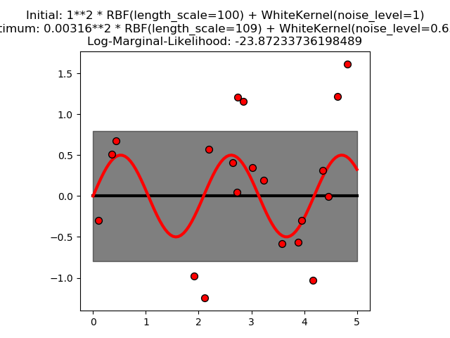
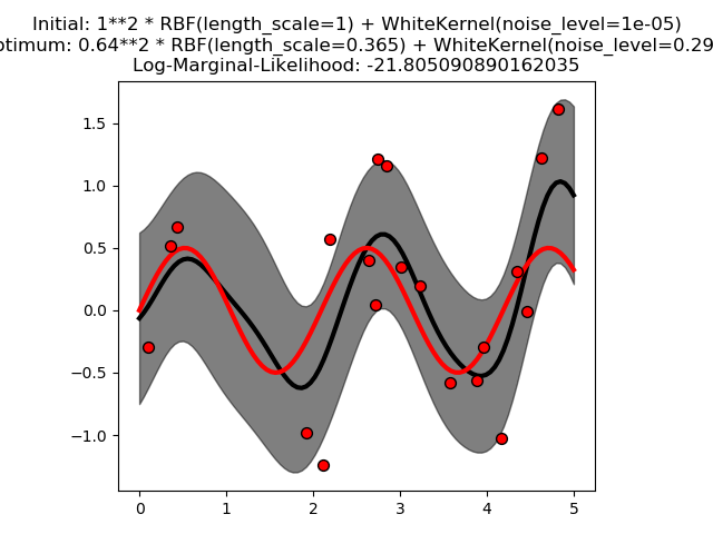
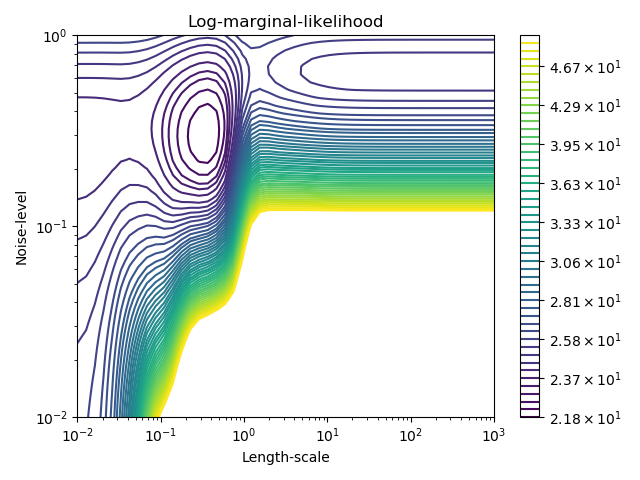
此示例说明具有和核(包括WhiteKernel)的CPR可以估计数据的噪声水平。对数边际似然(LML)的图的表明,LML存在两个局部极大值。第一个对应于一个高噪声级和大长度尺度的模型,它解释了数据中的所有噪声引起的变化。第二个噪声水平较小,长度尺度较短,解释了大部分的变化都是由无噪音的函数关系造成的。第二种模型具有较高的似然,然而,根据超参数的初始值,基于梯度的优化也可能收敛到高噪声的解。因此,对于不同的初始化,多次重复优化是很重要的。
print(__doc__)

# Authors: Jan Hendrik Metzen <jhm@informatik.uni-bremen.de>
#
# License: BSD 3 clause

import numpy as np

from matplotlib import pyplot as plt
from matplotlib.colors import LogNorm

from sklearn.gaussian_process import GaussianProcessRegressor
from sklearn.gaussian_process.kernels import RBF, WhiteKernel


rng = np.random.RandomState(0)
X = rng.uniform(0, 5, 20)[:, np.newaxis]
y = 0.5 * np.sin(3 * X[:, 0]) + rng.normal(0, 0.5, X.shape[0])

# First run
plt.figure()
kernel = 1.0 * RBF(length_scale=100.0, length_scale_bounds=(1e-2, 1e3)) \
    + WhiteKernel(noise_level=1, noise_level_bounds=(1e-10, 1e+1))
gp = GaussianProcessRegressor(kernel=kernel,
                              alpha=0.0).fit(X, y)
X_ = np.linspace(0, 5, 100)
y_mean, y_cov = gp.predict(X_[:, np.newaxis], return_cov=True)
plt.plot(X_, y_mean, 'k', lw=3, zorder=9)
plt.fill_between(X_, y_mean - np.sqrt(np.diag(y_cov)),
                 y_mean + np.sqrt(np.diag(y_cov)),
                 alpha=0.5, color='k')
plt.plot(X_, 0.5*np.sin(3*X_), 'r', lw=3, zorder=9)
plt.scatter(X[:, 0], y, c='r', s=50, zorder=10, edgecolors=(0, 0, 0))
plt.title("Initial: %s\nOptimum: %s\nLog-Marginal-Likelihood: %s"
          % (kernel, gp.kernel_,
             gp.log_marginal_likelihood(gp.kernel_.theta)))
plt.tight_layout()

# Second run
plt.figure()
kernel = 1.0 * RBF(length_scale=1.0, length_scale_bounds=(1e-2, 1e3)) \
    + WhiteKernel(noise_level=1e-5, noise_level_bounds=(1e-10, 1e+1))
gp = GaussianProcessRegressor(kernel=kernel,
                              alpha=0.0).fit(X, y)
X_ = np.linspace(0, 5, 100)
y_mean, y_cov = gp.predict(X_[:, np.newaxis], return_cov=True)
plt.plot(X_, y_mean, 'k', lw=3, zorder=9)
plt.fill_between(X_, y_mean - np.sqrt(np.diag(y_cov)),
                 y_mean + np.sqrt(np.diag(y_cov)),
                 alpha=0.5, color='k')
plt.plot(X_, 0.5*np.sin(3*X_), 'r', lw=3, zorder=9)
plt.scatter(X[:, 0], y, c='r', s=50, zorder=10, edgecolors=(0, 0, 0))
plt.title("Initial: %s\nOptimum: %s\nLog-Marginal-Likelihood: %s"
          % (kernel, gp.kernel_,
             gp.log_marginal_likelihood(gp.kernel_.theta)))
plt.tight_layout()

# Plot LML landscape
plt.figure()
theta0 = np.logspace(-2, 3, 49)
theta1 = np.logspace(-2, 0, 50)
Theta0, Theta1 = np.meshgrid(theta0, theta1)
LML = [[gp.log_marginal_likelihood(np.log([0.36, Theta0[i, j], Theta1[i, j]]))
        for i in range(Theta0.shape[0])] for j in range(Theta0.shape[1])]
LML = np.array(LML).T

vmin, vmax = (-LML).min(), (-LML).max()
vmax = 50
level = np.around(np.logspace(np.log10(vmin), np.log10(vmax), 50), decimals=1)
plt.contour(Theta0, Theta1, -LML,
            levels=level, norm=LogNorm(vmin=vmin, vmax=vmax))
plt.colorbar()
plt.xscale("log")
plt.yscale("log")
plt.xlabel("Length-scale")
plt.ylabel("Noise-level")
plt.title("Log-marginal-likelihood")
plt.tight_layout()

plt.show()
脚本的总运行时间:(0分3.520秒)

