

高斯过程回归:基本介绍性示例
一个简单的一维回归示例以两种不同的方式计算:
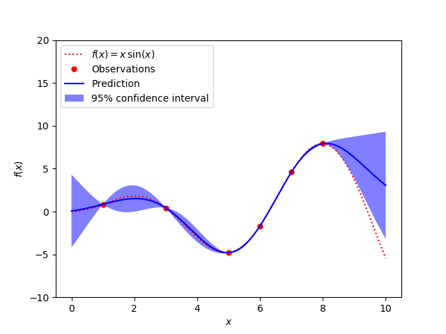
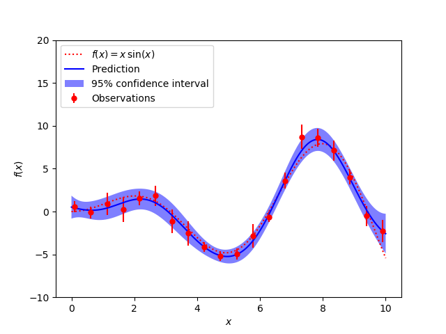
无噪声的情况 每个数据点都具有已知噪声级的噪声情况
在这两种情况下,核参数的估计使用最大似然原理。
图中以点态95%置信区间的形式说明了高斯过程模型的插值性质及其概率性质。
注意,参数alpha作为训练点之间假定协方差的Tikhonov正则化。
print(__doc__)

# Author: Vincent Dubourg <vincent.dubourg@gmail.com>
#         Jake Vanderplas <vanderplas@astro.washington.edu>
#         Jan Hendrik Metzen <jhm@informatik.uni-bremen.de>s
# License: BSD 3 clause

import numpy as np
from matplotlib import pyplot as plt

from sklearn.gaussian_process import GaussianProcessRegressor
from sklearn.gaussian_process.kernels import RBF, ConstantKernel as C

np.random.seed(1)


def f(x):
    """The function to predict."""
    return x * np.sin(x)

# ----------------------------------------------------------------------
#  First the noiseless case
X = np.atleast_2d([1., 3., 5., 6., 7., 8.]).T

# Observations
y = f(X).ravel()

# Mesh the input space for evaluations of the real function, the prediction and
# its MSE
x = np.atleast_2d(np.linspace(0, 10, 1000)).T

# Instantiate a Gaussian Process model
kernel = C(1.0, (1e-3, 1e3)) * RBF(10, (1e-2, 1e2))
gp = GaussianProcessRegressor(kernel=kernel, n_restarts_optimizer=9)

# Fit to data using Maximum Likelihood Estimation of the parameters
gp.fit(X, y)

# Make the prediction on the meshed x-axis (ask for MSE as well)
y_pred, sigma = gp.predict(x, return_std=True)

# Plot the function, the prediction and the 95% confidence interval based on
# the MSE
plt.figure()
plt.plot(x, f(x), 'r:', label=r'$f(x) = x\,\sin(x)$')
plt.plot(X, y, 'r.', markersize=10, label='Observations')
plt.plot(x, y_pred, 'b-', label='Prediction')
plt.fill(np.concatenate([x, x[::-1]]),
         np.concatenate([y_pred - 1.9600 * sigma,
                        (y_pred + 1.9600 * sigma)[::-1]]),
         alpha=.5, fc='b', ec='None', label='95% confidence interval')
plt.xlabel('$x$')
plt.ylabel('$f(x)$')
plt.ylim(-10, 20)
plt.legend(loc='upper left')

# ----------------------------------------------------------------------
# now the noisy case
X = np.linspace(0.1, 9.9, 20)
X = np.atleast_2d(X).T

# Observations and noise
y = f(X).ravel()
dy = 0.5 + 1.0 * np.random.random(y.shape)
noise = np.random.normal(0, dy)
y += noise

# Instantiate a Gaussian Process model
gp = GaussianProcessRegressor(kernel=kernel, alpha=dy ** 2,
                              n_restarts_optimizer=10)

# Fit to data using Maximum Likelihood Estimation of the parameters
gp.fit(X, y)

# Make the prediction on the meshed x-axis (ask for MSE as well)
y_pred, sigma = gp.predict(x, return_std=True)

# Plot the function, the prediction and the 95% confidence interval based on
# the MSE
plt.figure()
plt.plot(x, f(x), 'r:', label=r'$f(x) = x\,\sin(x)$')
plt.errorbar(X.ravel(), y, dy, fmt='r.', markersize=10, label='Observations')
plt.plot(x, y_pred, 'b-', label='Prediction')
plt.fill(np.concatenate([x, x[::-1]]),
         np.concatenate([y_pred - 1.9600 * sigma,
                        (y_pred + 1.9600 * sigma)[::-1]]),
         alpha=.5, fc='b', ec='None', label='95% confidence interval')
plt.xlabel('$x$')
plt.ylabel('$f(x)$')
plt.ylim(-10, 20)
plt.legend(loc='upper left')

plt.show()
脚本的总运行时间:(0分0.478秒)

