

核岭回归与高斯过程回归的比较
核岭回归(KRR)和高斯过程回归(GPR)都是通过内部使用“核技巧”来学习目标函数的。KRR在相应的核催生的空间中学习一个线性函数,该函数对应于原始空间中的一个非线性函数。线性函数的选择是基于带岭正则的军方误差损失。GPR使用核来定义目标函数的先验分布的协方差,并使用观测到的训练数据来定义似然函数。基于Bayes定理,定义了目标函数上的(高斯)后验分布,其均值用于预测。
一个主要的区别是,GPR可以基于边际似然函数的梯度上升来选择核的超参数,而KRR则需要对交叉验证的损失函数(均方误差损失)执行网格搜索。另一个不同之处是,GPR学习目标函数的生成概率模型,因此可以提供有意义的置信区间和后验样本以及预测,而KRR只提供预测。
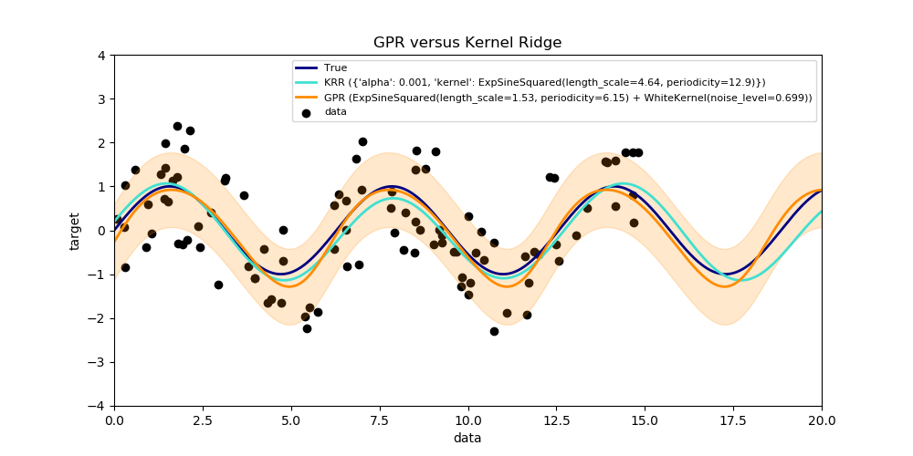
此示例说明了人工数据集上的这两种方法,该数据集由一个正弦目标函数和强噪声组成。图中比较了KRR和GPR学习到模型, 基于的是ExpSineSquared核, 这个核适用于学习周期函数。核的超参数控制核的光滑性(L)和周期性(P)。此外,数据的噪声水平是由GPR通过内核中附加的WhiteKernel成分和KRR的正则化参数α显式地学习的。
此图显示,这两种方法都学习了目标函数的合理模型。GPR正确地识别出函数的周期约为2*pi(6.28),而KRR选择的双倍的周期为4*pi。此外, GPR为预测提供了合理的置信界限, 但是KRR没有不能获取。这两种方法的一个主要区别是拟合和预测所需的时间:虽然拟合KRR在原则上是快速的,但网格搜索的超参数优化规模与超参数的数量成指数关系(“维数诅咒”)。在GPR中基于梯度的参数优化不会遭受这种指数尺度的影响, 因此在这个具有三维超参数空间的例子中,速度要快得多。然而,预测的时间是相似的,GPR产生预测分布的方差要比仅仅预测平均值花费的时间要长得多。
Time for KRR fitting: 4.593
Time for GPR fitting: 0.105
Time for KRR prediction: 0.054
Time for GPR prediction: 0.078
Time for GPR prediction with standard-deviation: 0.084
print(__doc__)

# Authors: Jan Hendrik Metzen <jhm@informatik.uni-bremen.de>
# License: BSD 3 clause


import time

import numpy as np

import matplotlib.pyplot as plt

from sklearn.kernel_ridge import KernelRidge
from sklearn.model_selection import GridSearchCV
from sklearn.gaussian_process import GaussianProcessRegressor
from sklearn.gaussian_process.kernels import WhiteKernel, ExpSineSquared

rng = np.random.RandomState(0)

# Generate sample data
X = 15 * rng.rand(100, 1)
y = np.sin(X).ravel()
y += 3 * (0.5 - rng.rand(X.shape[0]))  # add noise

# Fit KernelRidge with parameter selection based on 5-fold cross validation
param_grid = {"alpha": [1e0, 1e-1, 1e-2, 1e-3],
              "kernel": [ExpSineSquared(l, p)
                         for l in np.logspace(-2, 2, 10)
                         for p in np.logspace(0, 2, 10)]}
kr = GridSearchCV(KernelRidge(), param_grid=param_grid)
stime = time.time()
kr.fit(X, y)
print("Time for KRR fitting: %.3f" % (time.time() - stime))

gp_kernel = ExpSineSquared(1.0, 5.0, periodicity_bounds=(1e-2, 1e1)) \
    + WhiteKernel(1e-1)
gpr = GaussianProcessRegressor(kernel=gp_kernel)
stime = time.time()
gpr.fit(X, y)
print("Time for GPR fitting: %.3f" % (time.time() - stime))

# Predict using kernel ridge
X_plot = np.linspace(0, 20, 10000)[:, None]
stime = time.time()
y_kr = kr.predict(X_plot)
print("Time for KRR prediction: %.3f" % (time.time() - stime))

# Predict using gaussian process regressor
stime = time.time()
y_gpr = gpr.predict(X_plot, return_std=False)
print("Time for GPR prediction: %.3f" % (time.time() - stime))

stime = time.time()
y_gpr, y_std = gpr.predict(X_plot, return_std=True)
print("Time for GPR prediction with standard-deviation: %.3f"
      % (time.time() - stime))

# Plot results
plt.figure(figsize=(10, 5))
lw = 2
plt.scatter(X, y, c='k', label='data')
plt.plot(X_plot, np.sin(X_plot), color='navy', lw=lw, label='True')
plt.plot(X_plot, y_kr, color='turquoise', lw=lw,
         label='KRR (%s)' % kr.best_params_)
plt.plot(X_plot, y_gpr, color='darkorange', lw=lw,
         label='GPR (%s)' % gpr.kernel_)
plt.fill_between(X_plot[:, 0], y_gpr - y_std, y_gpr + y_std, color='darkorange',
                 alpha=0.2)
plt.xlabel('data')
plt.ylabel('target')
plt.xlim(0, 20)
plt.ylim(-4, 4)
plt.title('GPR versus Kernel Ridge')
plt.legend(loc="best",  scatterpoints=1, prop={'size': 8})
plt.show()
脚本的总运行时间:(0分5.065秒)

