

在iris数据集上的高斯过程分类
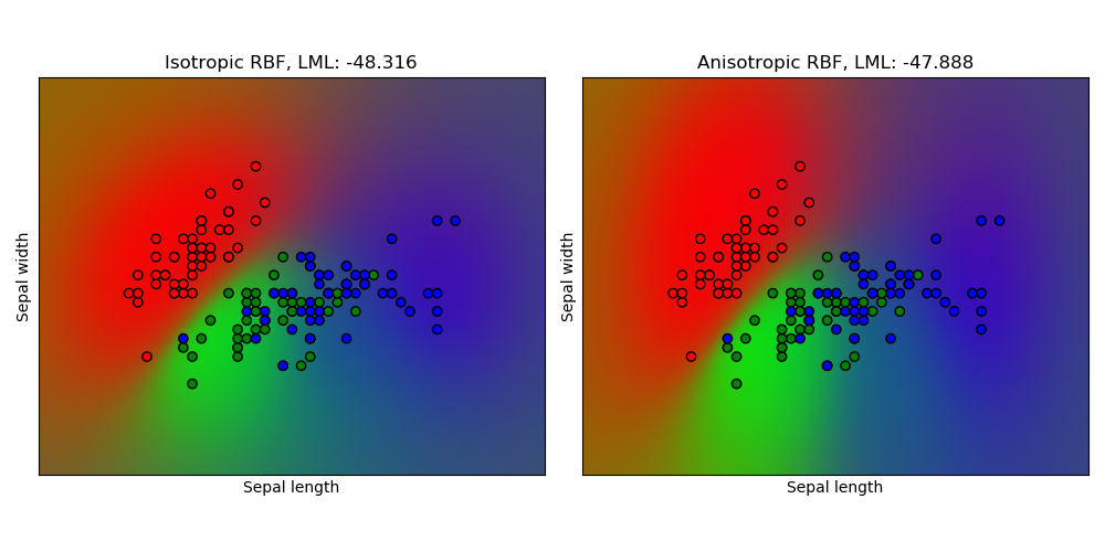
这个例子说明了在二维版本的iris数据集上,各向同性和各向异性径向基函数核(RBF)的GPC的预测概率。各向异性径向基函数核通过给两个特征维分配不同的长度尺度,得到略高的对数边际似然。
print(__doc__)

import numpy as np
import matplotlib.pyplot as plt
from sklearn import datasets
from sklearn.gaussian_process import GaussianProcessClassifier
from sklearn.gaussian_process.kernels import RBF

# import some data to play with
iris = datasets.load_iris()
X = iris.data[:, :2]  # we only take the first two features.
y = np.array(iris.target, dtype=int)

h = .02  # step size in the mesh

kernel = 1.0 * RBF([1.0])
gpc_rbf_isotropic = GaussianProcessClassifier(kernel=kernel).fit(X, y)
kernel = 1.0 * RBF([1.0, 1.0])
gpc_rbf_anisotropic = GaussianProcessClassifier(kernel=kernel).fit(X, y)

# create a mesh to plot in
x_min, x_max = X[:, 0].min() - 1, X[:, 0].max() + 1
y_min, y_max = X[:, 1].min() - 1, X[:, 1].max() + 1
xx, yy = np.meshgrid(np.arange(x_min, x_max, h),
                     np.arange(y_min, y_max, h))

titles = ["Isotropic RBF", "Anisotropic RBF"]
plt.figure(figsize=(10, 5))
for i, clf in enumerate((gpc_rbf_isotropic, gpc_rbf_anisotropic)):
    # Plot the predicted probabilities. For that, we will assign a color to
    # each point in the mesh [x_min, m_max]x[y_min, y_max].
    plt.subplot(1, 2, i + 1)

    Z = clf.predict_proba(np.c_[xx.ravel(), yy.ravel()])

    # Put the result into a color plot
    Z = Z.reshape((xx.shape[0], xx.shape[1], 3))
    plt.imshow(Z, extent=(x_min, x_max, y_min, y_max), origin="lower")

    # Plot also the training points
    plt.scatter(X[:, 0], X[:, 1], c=np.array(["r", "g", "b"])[y],
                edgecolors=(0, 0, 0))
    plt.xlabel('Sepal length')
    plt.ylabel('Sepal width')
    plt.xlim(xx.min(), xx.max())
    plt.ylim(yy.min(), yy.max())
    plt.xticks(())
    plt.yticks(())
    plt.title("%s, LML: %.3f" %
              (titles[i], clf.log_marginal_likelihood(clf.kernel_.theta)))

plt.tight_layout()
plt.show()
脚本的总运行时间:(0分3.967秒)

