

高斯混合模型选择
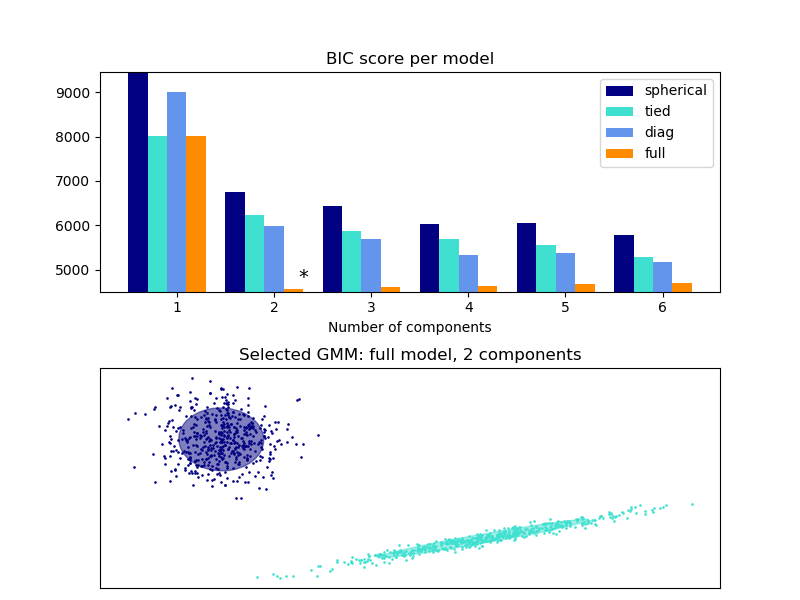
实例表明,利用信息论准则(BIC)可以对高斯混合模型进行模型选择。模型选择涉及到模型中的协方差类型和成分数。在这种情况下,AIC也提供了正确的结果(没有显示出来以节省时间),但是如果问题是确定正确的模型,则BIC更适合。与贝叶斯程序不同的是,这种推断是无先验的。
在这种情况下,选择具有两个成分和完全协方差(对应于真实生成模型)的模型。
import numpy as np
import itertools

from scipy import linalg
import matplotlib.pyplot as plt
import matplotlib as mpl

from sklearn import mixture

print(__doc__)

# Number of samples per component
n_samples = 500

# Generate random sample, two components
np.random.seed(0)
C = np.array([[0., -0.1], [1.7, .4]])
X = np.r_[np.dot(np.random.randn(n_samples, 2), C),
          .7 * np.random.randn(n_samples, 2) + np.array([-6, 3])]

lowest_bic = np.infty
bic = []
n_components_range = range(1, 7)
cv_types = ['spherical', 'tied', 'diag', 'full']
for cv_type in cv_types:
    for n_components in n_components_range:
        # Fit a Gaussian mixture with EM
        gmm = mixture.GaussianMixture(n_components=n_components,
                                      covariance_type=cv_type)
        gmm.fit(X)
        bic.append(gmm.bic(X))
        if bic[-1] < lowest_bic:
            lowest_bic = bic[-1]
            best_gmm = gmm

bic = np.array(bic)
color_iter = itertools.cycle(['navy', 'turquoise', 'cornflowerblue',
                              'darkorange'])
clf = best_gmm
bars = []

# Plot the BIC scores
plt.figure(figsize=(8, 6))
spl = plt.subplot(2, 1, 1)
for i, (cv_type, color) in enumerate(zip(cv_types, color_iter)):
    xpos = np.array(n_components_range) + .2 * (i - 2)
    bars.append(plt.bar(xpos, bic[i * len(n_components_range):
                                  (i + 1) * len(n_components_range)],
                        width=.2, color=color))
plt.xticks(n_components_range)
plt.ylim([bic.min() * 1.01 - .01 * bic.max(), bic.max()])
plt.title('BIC score per model')
xpos = np.mod(bic.argmin(), len(n_components_range)) + .65 +\
    .2 * np.floor(bic.argmin() / len(n_components_range))
plt.text(xpos, bic.min() * 0.97 + .03 * bic.max(), '*', fontsize=14)
spl.set_xlabel('Number of components')
spl.legend([b[0] for b in bars], cv_types)

# Plot the winner
splot = plt.subplot(2, 1, 2)
Y_ = clf.predict(X)
for i, (mean, cov, color) in enumerate(zip(clf.means_, clf.covariances_,
                                           color_iter)):
    v, w = linalg.eigh(cov)
    if not np.any(Y_ == i):
        continue
    plt.scatter(X[Y_ == i, 0], X[Y_ == i, 1], .8, color=color)

    # Plot an ellipse to show the Gaussian component
    angle = np.arctan2(w[0][1], w[0][0])
    angle = 180. * angle / np.pi  # convert to degrees
    v = 2. * np.sqrt(2.) * np.sqrt(v)
    ell = mpl.patches.Ellipse(mean, v[0], v[1], 180. + angle, color=color)
    ell.set_clip_box(splot.bbox)
    ell.set_alpha(.5)
    splot.add_artist(ell)

plt.xticks(())
plt.yticks(())
plt.title('Selected GMM: full model, 2 components')
plt.subplots_adjust(hspace=.35, bottom=.02)
plt.show()
脚本的总运行时间:(0分0.458秒)

