基于概率主成分分析和因子分析(FA)的模型选择¶

概率PCA和因子分析是概率模型。其结果是，新数据的似然可用于模型选择和协方差估计。在这里，我们使用交叉验证在低秩的被破坏的同方差噪声数据上比较了PCA和FA(每个特征的噪声方差是相同的)或异方差噪声(每个特征的噪声方差是不同的)。在第二步，我们比较了模型从收缩协方差估计得到的似然。

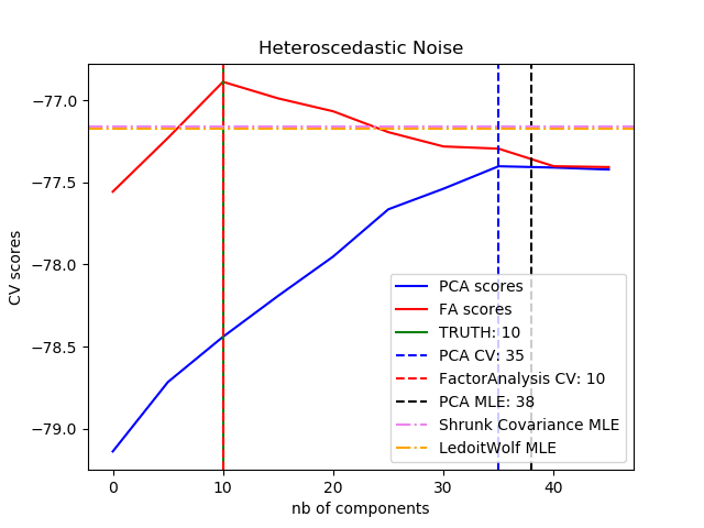
可以观察到，在同方差噪声下，FA和PCA都成功地恢复了低秩子空间的大小。在这种情况下，PCA的似然高于FA。然而，当存在异方差噪声时，PCA失败并高估了秩。在适当的情况下，低秩模型比收缩模型更有可能出现。

PCA维数自动选择的自动估计。NIP 2000：598-604由ThomasP.Minka也做了比较。

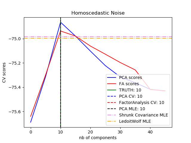
best n_components by PCA CV = 10
best n_components by FactorAnalysis CV = 10
best n_components by PCA MLE = 10
best n_components by PCA CV = 35
best n_components by FactorAnalysis CV = 10
best n_components by PCA MLE = 38

# Authors: Alexandre Gramfort
#          Denis A. Engemann
# License: BSD 3 clause

import numpy as np
import matplotlib.pyplot as plt
from scipy import linalg

from sklearn.decomposition import PCA, FactorAnalysis
from sklearn.covariance import ShrunkCovariance, LedoitWolf
from sklearn.model_selection import cross_val_score
from sklearn.model_selection import GridSearchCV

print(__doc__)

# #############################################################################
# Create the data

n_samples, n_features, rank = 1000, 50, 10
sigma = 1.
rng = np.random.RandomState(42)
U, _, _ = linalg.svd(rng.randn(n_features, n_features))
X = np.dot(rng.randn(n_samples, rank), U[:, :rank].T)

# Adding homoscedastic noise
X_homo = X + sigma * rng.randn(n_samples, n_features)

# Adding heteroscedastic noise
sigmas = sigma * rng.rand(n_features) + sigma / 2.
X_hetero = X + rng.randn(n_samples, n_features) * sigmas

# #############################################################################
# Fit the models

n_components = np.arange(0, n_features, 5)  # options for n_components


def compute_scores(X):
    pca = PCA(svd_solver='full')
    fa = FactorAnalysis()

    pca_scores, fa_scores = [], []
    for n in n_components:
        pca.n_components = n
        fa.n_components = n
        pca_scores.append(np.mean(cross_val_score(pca, X)))
        fa_scores.append(np.mean(cross_val_score(fa, X)))

    return pca_scores, fa_scores


def shrunk_cov_score(X):
    shrinkages = np.logspace(-2, 0, 30)
    cv = GridSearchCV(ShrunkCovariance(), {'shrinkage': shrinkages})
    return np.mean(cross_val_score(cv.fit(X).best_estimator_, X))


def lw_score(X):
    return np.mean(cross_val_score(LedoitWolf(), X))


for X, title in [(X_homo, 'Homoscedastic Noise'),
                 (X_hetero, 'Heteroscedastic Noise')]:
    pca_scores, fa_scores = compute_scores(X)
    n_components_pca = n_components[np.argmax(pca_scores)]
    n_components_fa = n_components[np.argmax(fa_scores)]

    pca = PCA(svd_solver='full', n_components='mle')
    pca.fit(X)
    n_components_pca_mle = pca.n_components_

    print("best n_components by PCA CV = %d" % n_components_pca)
    print("best n_components by FactorAnalysis CV = %d" % n_components_fa)
    print("best n_components by PCA MLE = %d" % n_components_pca_mle)

    plt.figure()
    plt.plot(n_components, pca_scores, 'b', label='PCA scores')
    plt.plot(n_components, fa_scores, 'r', label='FA scores')
    plt.axvline(rank, color='g', label='TRUTH: %d' % rank, linestyle='-')
    plt.axvline(n_components_pca, color='b',
                label='PCA CV: %d' % n_components_pca, linestyle='--')
    plt.axvline(n_components_fa, color='r',
                label='FactorAnalysis CV: %d' % n_components_fa,
                linestyle='--')
    plt.axvline(n_components_pca_mle, color='k',
                label='PCA MLE: %d' % n_components_pca_mle, linestyle='--')

    # compare with other covariance estimators
    plt.axhline(shrunk_cov_score(X), color='violet',
                label='Shrunk Covariance MLE', linestyle='-.')
    plt.axhline(lw_score(X), color='orange',
                label='LedoitWolf MLE' % n_components_pca_mle, linestyle='-.')

    plt.xlabel('nb of components')
    plt.ylabel('CV scores')
    plt.legend(loc='lower right')
    plt.title(title)

plt.show()

脚本的总运行时间：(0分10.802秒)

Download Python source code:plot_pca_vs_fa_model_selection.py

Download Jupyter notebook:plot_pca_vs_fa_model_selection.ipynb