

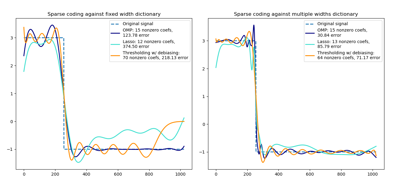
使用预计算字典的稀疏编码
将信号变换为Ricker小波的稀疏组合。这个例子直观地比较了不同的稀疏编码方法, 使用sklearn.decomposition.SparseCoder 估计器。Ricker(也称为Mexican hat或高斯的二阶导数)不是一个特别好的内核,可以表示像这样的分段常量信号。因此,我们可以看到增加了多少微量的不同宽度,并且因此它激发了学习字典,以最适合你的信号类型。
右边较丰富的字典的尺寸并不大,较重的子抽样是为了保持相同的数量级。
print(__doc__)

from distutils.version import LooseVersion

import numpy as np
import matplotlib.pyplot as plt

from sklearn.decomposition import SparseCoder


def ricker_function(resolution, center, width):
    """Discrete sub-sampled Ricker (Mexican hat) wavelet"""
    x = np.linspace(0, resolution - 1, resolution)
    x = ((2 / (np.sqrt(3 * width) * np.pi ** .25))
         * (1 - (x - center) ** 2 / width ** 2)
         * np.exp(-(x - center) ** 2 / (2 * width ** 2)))
    return x


def ricker_matrix(width, resolution, n_components):
    """Dictionary of Ricker (Mexican hat) wavelets"""
    centers = np.linspace(0, resolution - 1, n_components)
    D = np.empty((n_components, resolution))
    for i, center in enumerate(centers):
        D[i] = ricker_function(resolution, center, width)
    D /= np.sqrt(np.sum(D ** 2, axis=1))[:, np.newaxis]
    return D


resolution = 1024
subsampling = 3  # subsampling factor
width = 100
n_components = resolution // subsampling

# Compute a wavelet dictionary
D_fixed = ricker_matrix(width=width, resolution=resolution,
                        n_components=n_components)
D_multi = np.r_[tuple(ricker_matrix(width=w, resolution=resolution,
                      n_components=n_components // 5)
                for w in (10, 50, 100, 500, 1000))]

# Generate a signal
y = np.linspace(0, resolution - 1, resolution)
first_quarter = y < resolution / 4
y[first_quarter] = 3.
y[np.logical_not(first_quarter)] = -1.

# List the different sparse coding methods in the following format:
# (title, transform_algorithm, transform_alpha,
#  transform_n_nozero_coefs, color)
estimators = [('OMP', 'omp', None, 15, 'navy'),
              ('Lasso', 'lasso_lars', 2, None, 'turquoise'), ]
lw = 2
# Avoid FutureWarning about default value change when numpy >= 1.14
lstsq_rcond = None if LooseVersion(np.__version__) >= '1.14' else -1

plt.figure(figsize=(13, 6))
for subplot, (D, title) in enumerate(zip((D_fixed, D_multi),
                                         ('fixed width', 'multiple widths'))):
    plt.subplot(1, 2, subplot + 1)
    plt.title('Sparse coding against %s dictionary' % title)
    plt.plot(y, lw=lw, linestyle='--', label='Original signal')
    # Do a wavelet approximation
    for title, algo, alpha, n_nonzero, color in estimators:
        coder = SparseCoder(dictionary=D, transform_n_nonzero_coefs=n_nonzero,
                            transform_alpha=alpha, transform_algorithm=algo)
        x = coder.transform(y.reshape(1, -1))
        density = len(np.flatnonzero(x))
        x = np.ravel(np.dot(x, D))
        squared_error = np.sum((y - x) ** 2)
        plt.plot(x, color=color, lw=lw,
                 label='%s: %s nonzero coefs,\n%.2f error'
                 % (title, density, squared_error))

    # Soft thresholding debiasing
    coder = SparseCoder(dictionary=D, transform_algorithm='threshold',
                        transform_alpha=20)
    x = coder.transform(y.reshape(1, -1))
    _, idx = np.where(x != 0)
    x[0, idx], _, _, _ = np.linalg.lstsq(D[idx, :].T, y, rcond=lstsq_rcond)
    x = np.ravel(np.dot(x, D))
    squared_error = np.sum((y - x) ** 2)
    plt.plot(x, color='darkorange', lw=lw,
             label='Thresholding w/ debiasing:\n%d nonzero coefs, %.2f error'
             % (len(idx), squared_error))
    plt.axis('tight')
    plt.legend(shadow=False, loc='best')
plt.subplots_adjust(.04, .07, .97, .90, .09, .2)
plt.show()
脚本的总运行时间:(0分0.380秒)

