

用于数字分类的‘受限玻尔兹曼机’功能
对于灰度图像数据,其中像素值可以解释为白色背景上的黑度,例如手写数字识别,Bernoulli受限Boltzmann机器模型(BernoulliRBM)可以执行有效的非线性特征提取。
为了从一个小的数据集中学到良好的潜在表示,我们通过在每个方向上线性移动1个像素的扰动训练数据来人工生成更多的标记数据。
本示例说明如何使用BernoulliRBM特征提取器和LogisticRegression分类器构建分类管道。 整个模型的超参数(学习率,隐藏层大小,正则化)已通过网格搜索进行了优化,但由于运行时限制,此处未复制搜索。
提出了对原始像素值的逻辑回归以进行比较。 该示例表明,BernoulliRBM提取的特征有助于提高分类准确性。
print(__doc__)
# 作者: Yann N. Dauphin, Vlad Niculae, Gabriel Synnaeve
# 执照: BSD
import numpy as np
import matplotlib.pyplot as plt
from scipy.ndimage import convolve
from sklearn import linear_model, datasets, metrics
from sklearn.model_selection import train_test_split
from sklearn.neural_network import BernoulliRBM
from sklearn.pipeline import Pipeline
from sklearn.base import clone
# #############################################################################
# Setting up
def nudge_dataset(X, Y):
"""
将X中的8x8图像左右,左右,向下,向上移动1px
这样产生的数据集比原始数据集大5倍
"""
direction_vectors = [
[[0, 1, 0],
[0, 0, 0],
[0, 0, 0]],
[[0, 0, 0],
[1, 0, 0],
[0, 0, 0]],
[[0, 0, 0],
[0, 0, 1],
[0, 0, 0]],
[[0, 0, 0],
[0, 0, 0],
[0, 1, 0]]]
def shift(x, w):
return convolve(x.reshape((8, 8)), mode='constant', weights=w).ravel()
X = np.concatenate([X] +
[np.apply_along_axis(shift, 1, X, vector)
for vector in direction_vectors])
Y = np.concatenate([Y for _ in range(5)], axis=0)
return X, Y
# Load Data
X, y = datasets.load_digits(return_X_y=True)
X = np.asarray(X, 'float32')
X, Y = nudge_dataset(X, y)
X = (X - np.min(X, 0)) / (np.max(X, 0) + 0.0001) # 0-1 scaling
X_train, X_test, Y_train, Y_test = train_test_split(
X, Y, test_size=0.2, random_state=0)
# 我们要使用的模型:
logistic = linear_model.LogisticRegression(solver='newton-cg', tol=1)
rbm = BernoulliRBM(random_state=0, verbose=True)
rbm_features_classifier = Pipeline(
steps=[('rbm', rbm), ('logistic', logistic)])
# #############################################################################
# 训练
# 超参数,这些是使用GridSearchCV通过交叉验证设置的。
# 在这里,我们不执行交叉验证以节省时间。
rbm.learning_rate = 0.06
rbm.n_iter = 10
# 更多的组件倾向于提供更好的预测性能,但拟合时间更长
rbm.n_components = 100
logistic.C = 6000
# 培训RBM-Logistic管道
rbm_features_classifier.fit(X_train, Y_train)
# 直接在像素上训练Logistic回归分类器
raw_pixel_classifier = clone(logistic)
raw_pixel_classifier.C = 100.
raw_pixel_classifier.fit(X_train, Y_train)
# #############################################################################
# 评估
Y_pred = rbm_features_classifier.predict(X_test)
print("Logistic regression using RBM features:\n%s\n" % (
metrics.classification_report(Y_test, Y_pred)))
Y_pred = raw_pixel_classifier.predict(X_test)
print("Logistic regression using raw pixel features:\n%s\n" % (
metrics.classification_report(Y_test, Y_pred)))
# #############################################################################
# Plotting
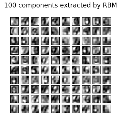
plt.figure(figsize=(4.2, 4))
for i, comp in enumerate(rbm.components_):
plt.subplot(10, 10, i + 1)
plt.imshow(comp.reshape((8, 8)), cmap=plt.cm.gray_r,
interpolation='nearest')
plt.xticks(())
plt.yticks(())
plt.suptitle('100 components extracted by RBM', fontsize=16)
plt.subplots_adjust(0.08, 0.02, 0.92, 0.85, 0.08, 0.23)
plt.show()
输出:
[BernoulliRBM] Iteration 1, pseudo-likelihood = -25.39, time = 0.26s
[BernoulliRBM] Iteration 2, pseudo-likelihood = -23.77, time = 0.35s
[BernoulliRBM] Iteration 3, pseudo-likelihood = -22.94, time = 0.35s
[BernoulliRBM] Iteration 4, pseudo-likelihood = -21.91, time = 0.35s
[BernoulliRBM] Iteration 5, pseudo-likelihood = -21.69, time = 0.34s
[BernoulliRBM] Iteration 6, pseudo-likelihood = -21.06, time = 0.35s
[BernoulliRBM] Iteration 7, pseudo-likelihood = -20.89, time = 0.34s
[BernoulliRBM] Iteration 8, pseudo-likelihood = -20.64, time = 0.36s
[BernoulliRBM] Iteration 9, pseudo-likelihood = -20.36, time = 0.35s
[BernoulliRBM] Iteration 10, pseudo-likelihood = -20.09, time = 0.34s
Logistic regression using RBM features:
              precision    recall  f1-score   support

           0       0.99      0.98      0.99       174
           1       0.91      0.93      0.92       184
           2       0.94      0.96      0.95       166
           3       0.96      0.90      0.93       194
           4       0.97      0.94      0.96       186
           5       0.91      0.92      0.92       181
           6       0.98      0.97      0.97       207
           7       0.94      0.98      0.96       154
           8       0.91      0.90      0.90       182
           9       0.87      0.91      0.89       169

    accuracy                           0.94      1797
   macro avg       0.94      0.94      0.94      1797
weighted avg       0.94      0.94      0.94      1797


Logistic regression using raw pixel features:
              precision    recall  f1-score   support

           0       0.90      0.92      0.91       174
           1       0.60      0.58      0.59       184
           2       0.76      0.85      0.80       166
           3       0.78      0.79      0.78       194
           4       0.82      0.84      0.83       186
           5       0.76      0.76      0.76       181
           6       0.90      0.87      0.89       207
           7       0.85      0.88      0.87       154
           8       0.67      0.58      0.62       182
           9       0.75      0.76      0.75       169

    accuracy                           0.78      1797
   macro avg       0.78      0.78      0.78      1797
weighted avg       0.78      0.78      0.78      1797
脚本的总运行时间:(0分钟8.949秒)

