训练误差与测试误差¶

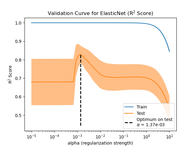
本案例可视化了估算器在未曾见过的数据（测试数据）上的性能与训练数据的性能如何不同。随着正则化的增加，训练集的性能会下降，而测试集上的性能在正则化参数的值范围内最佳。这是一个使用Elastic-Net回归模型、使用可解释性方差，即来衡量性能的案例。（译者注：可解释性方差与有同向数学关系，因此两者在某种意义上可以等同）

输出：

Optimal regularization parameter : 0.00013141473626117567

输入：

print(__doc__)

# 作者: Alexandre Gramfort <alexandre.gramfort@inria.fr>
# 执照: BSD 3 clause

import numpy as np
from sklearn import linear_model

# #############################################################################
# 获取样本信息
n_samples_train, n_samples_test, n_features = 75, 150, 500
np.random.seed(0)
coef = np.random.randn(n_features)
coef[50:] = 0.0  # 只有前10个特征会影响模型
X = np.random.randn(n_samples_train + n_samples_test, n_features)
y = np.dot(X, coef)

# 分割训练集与测试集
X_train, X_test = X[:n_samples_train], X[n_samples_train:]
y_train, y_test = y[:n_samples_train], y[n_samples_train:]

# #############################################################################
# 计算训练与测试误差
alphas = np.logspace(-5, 1, 60)
enet = linear_model.ElasticNet(l1_ratio=0.7, max_iter=10000)
train_errors = list()
test_errors = list()
for alpha in alphas:
    enet.set_params(alpha=alpha)
    enet.fit(X_train, y_train)
    train_errors.append(enet.score(X_train, y_train))
    test_errors.append(enet.score(X_test, y_test))

i_alpha_optim = np.argmax(test_errors)
alpha_optim = alphas[i_alpha_optim]
print("Optimal regularization parameter : %s" % alpha_optim)

# 使用最佳正则化参数估计完整数据上的coef_
enet.set_params(alpha=alpha_optim)
coef_ = enet.fit(X, y).coef_

# #############################################################################
# 绘制结果方程

import matplotlib.pyplot as plt
plt.subplot(2, 1, 1)
plt.semilogx(alphas, train_errors, label='Train')
plt.semilogx(alphas, test_errors, label='Test')
plt.vlines(alpha_optim, plt.ylim()[0], np.max(test_errors), color='k',
           linewidth=3, label='Optimum on test')
plt.legend(loc='lower left')
plt.ylim([0, 1.2])
plt.xlabel('Regularization parameter')
plt.ylabel('Performance')

# 展示预测的 coef_ 与真实的系数之间的差异
plt.subplot(2, 1, 2)
plt.plot(coef, label='True coef')
plt.plot(coef_, label='Estimated coef')
plt.legend()
plt.subplots_adjust(0.09, 0.04, 0.94, 0.94, 0.26, 0.26)
plt.show()

脚本的总运行时间：（0分钟2.662秒）