欠拟合与过拟合¶

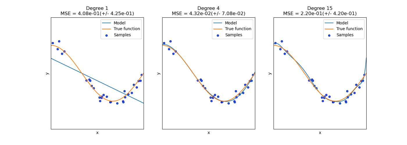
此案例展现了拟合不足和拟合过度的问题，以及如何使用具有多项式特征的线性回归来估计非线性函数。该图显示了我们要估计的函数，它是余弦函数的一部分。 此外，还将显示来自真实函数的样本以及不同模型的近似值。这些模型具有不同程度的多项式特征。我们可以看到线性函数（阶数为1的多项式）不足以拟合训练样本。 这称为欠拟合。4次多项式几乎完美地逼近了真实的函数。但是，对于较高的次数，模型将过度拟合训练数据，即模型会学习训练数据的噪声。我们通过使用交叉验证来定量评估过度拟合/不足拟合。我们在验证集上计算均方误差（MSE），该误差越高，模型从训练数据正确拟合、学到真实函数的可能性就越小。

print(__doc__)

import numpy as np
import matplotlib.pyplot as plt
from sklearn.pipeline import Pipeline
from sklearn.preprocessing import PolynomialFeatures
from sklearn.linear_model import LinearRegression
from sklearn.model_selection import cross_val_score


def true_fun(X):
    return np.cos(1.5 * np.pi * X)

np.random.seed(0)

n_samples = 30
degrees = [1, 4, 15]

X = np.sort(np.random.rand(n_samples))
y = true_fun(X) + np.random.randn(n_samples) * 0.1

plt.figure(figsize=(14, 5))
for i in range(len(degrees)):
    ax = plt.subplot(1, len(degrees), i + 1)
    plt.setp(ax, xticks=(), yticks=())

    polynomial_features = PolynomialFeatures(degree=degrees[i],
                                             include_bias=False)
    linear_regression = LinearRegression()
    pipeline = Pipeline([("polynomial_features", polynomial_features),
                         ("linear_regression", linear_regression)])
    pipeline.fit(X[:, np.newaxis], y)

    # Evaluate the models using crossvalidation
    scores = cross_val_score(pipeline, X[:, np.newaxis], y,
                             scoring="neg_mean_squared_error", cv=10)

    X_test = np.linspace(0, 1, 100)
    plt.plot(X_test, pipeline.predict(X_test[:, np.newaxis]), label="Model")
    plt.plot(X_test, true_fun(X_test), label="True function")
    plt.scatter(X, y, edgecolor='b', s=20, label="Samples")
    plt.xlabel("x")
    plt.ylabel("y")
    plt.xlim((0, 1))
    plt.ylim((-2, 2))
    plt.legend(loc="best")
    plt.title("Degree {}\nMSE = {:.2e}(+/- {:.2e})".format(
        degrees[i], -scores.mean(), scores.std()))
plt.show()

脚本的总运行时间：（0分钟0.229秒）