等渗回归¶

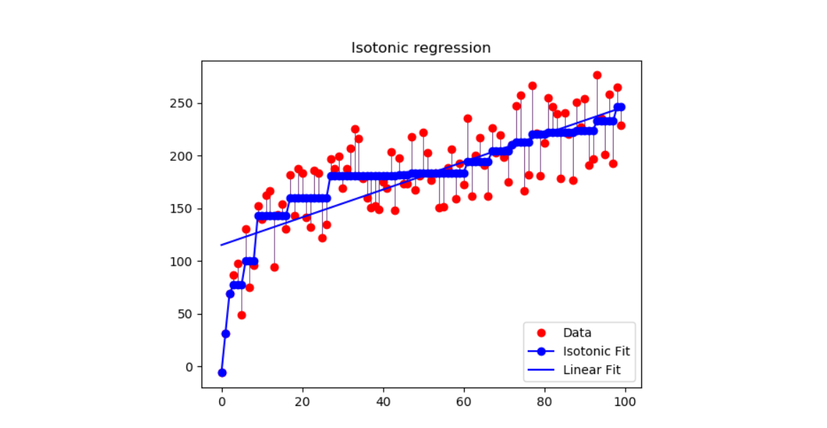
在生成的数据集上展示等身回归的用法。等渗回归会寻找函数的非递减近似，同时使训练数据的均方误差最小。 这种模型的好处是它不会对目标函数采用任何形式的假设，例如线性。为了比较，还使用了线性回归。

# 代码作者: Nelle Varoquaux <nelle.varoquaux@gmail.com>
#          Alexandre Gramfort <alexandre.gramfort@inria.fr>
# 执照: BSD

import numpy as np
import matplotlib.pyplot as plt
from matplotlib.collections import LineCollection

from sklearn.linear_model import LinearRegression
from sklearn.isotonic import IsotonicRegression
from sklearn.utils import check_random_state

n = 100
x = np.arange(n)
rs = check_random_state(0)
y = rs.randint(-50, 50, size=(n,)) + 50. * np.log1p(np.arange(n))

# #############################################################################
#拟合等渗回归和线性回归模型

ir = IsotonicRegression()

y_ = ir.fit_transform(x, y)

lr = LinearRegression()
lr.fit(x[:, np.newaxis], y)  #对线性回归而言X需要时二维的

# #############################################################################
# 绘制结果

segments = [[[i, y[i]], [i, y_[i]]] for i in range(n)]
lc = LineCollection(segments, zorder=0)
lc.set_array(np.ones(len(y)))
lc.set_linewidths(np.full(n, 0.5))

fig = plt.figure()
plt.plot(x, y, 'r.', markersize=12)
plt.plot(x, y_, 'b.-', markersize=12)
plt.plot(x, lr.predict(x[:, np.newaxis]), 'b-')
plt.gca().add_collection(lc)
plt.legend(('Data', 'Isotonic Fit', 'Linear Fit'), loc='lower right')
plt.title('Isotonic regression')
plt.show()

输出：

脚本的总运行时间：0分钟0.124秒