

单变量特征选择
一个显示单变量特征选择的例子。
在iris数据中加入含噪(非信息)特征,并采用单变量特征选择。对于每个特征,我们绘制了单变量特征选择的p-值和支持向量机的相应权重。我们可以看到,单变量特征选择选择了信息丰富的特征,并且这些特征具有较大的支持向量机权重。
在所有的特征集合中,只有前四个特征是显著的。我们可以看到,他们在单变量特征选择中得分最高。支持向量机为这些特征之一分配了很大的权重,但也选择了许多信息不丰富的特征。在支持向量机之前应用单变量特征选择,可以增加对显著特征的支持向量机的权重,从而改进分类。
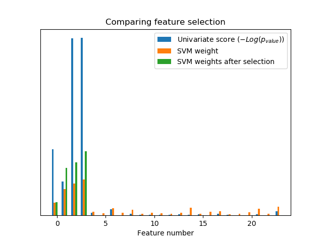
Classification accuracy without selecting features: 0.789
Classification accuracy after univariate feature selection: 0.868
print(__doc__)

import numpy as np
import matplotlib.pyplot as plt

from sklearn.datasets import load_iris
from sklearn.model_selection import train_test_split
from sklearn.preprocessing import MinMaxScaler
from sklearn.svm import LinearSVC
from sklearn.pipeline import make_pipeline
from sklearn.feature_selection import SelectKBest, f_classif

# #############################################################################
# Import some data to play with

# The iris dataset
X, y = load_iris(return_X_y=True)

# Some noisy data not correlated
E = np.random.RandomState(42).uniform(0, 0.1, size=(X.shape[0], 20))

# Add the noisy data to the informative features
X = np.hstack((X, E))

# Split dataset to select feature and evaluate the classifier
X_train, X_test, y_train, y_test = train_test_split(
        X, y, stratify=y, random_state=0
)

plt.figure(1)
plt.clf()

X_indices = np.arange(X.shape[-1])

# #############################################################################
# Univariate feature selection with F-test for feature scoring
# We use the default selection function to select the four
# most significant features
selector = SelectKBest(f_classif, k=4)
selector.fit(X_train, y_train)
scores = -np.log10(selector.pvalues_)
scores /= scores.max()
plt.bar(X_indices - .45, scores, width=.2,
        label=r'Univariate score ($-Log(p_{value})$)')

# #############################################################################
# Compare to the weights of an SVM
clf = make_pipeline(MinMaxScaler(), LinearSVC())
clf.fit(X_train, y_train)
print('Classification accuracy without selecting features: {:.3f}'
      .format(clf.score(X_test, y_test)))

svm_weights = np.abs(clf[-1].coef_).sum(axis=0)
svm_weights /= svm_weights.sum()

plt.bar(X_indices - .25, svm_weights, width=.2, label='SVM weight')

clf_selected = make_pipeline(
        SelectKBest(f_classif, k=4), MinMaxScaler(), LinearSVC()
)
clf_selected.fit(X_train, y_train)
print('Classification accuracy after univariate feature selection: {:.3f}'
      .format(clf_selected.score(X_test, y_test)))

svm_weights_selected = np.abs(clf_selected[-1].coef_).sum(axis=0)
svm_weights_selected /= svm_weights_selected.sum()

plt.bar(X_indices[selector.get_support()] - .05, svm_weights_selected,
        width=.2, label='SVM weights after selection')


plt.title("Comparing feature selection")
plt.xlabel('Feature number')
plt.yticks(())
plt.axis('tight')
plt.legend(loc='upper right')
plt.show()
脚本的总运行时间:(0分0.139秒)

