

稳健与经验协方差估计
通常的协方差极大似然估计对数据集中异常值的存在非常敏感。在这种情况下,最好使用稳健的协方差估计器,以确保估计能够抵抗数据集中的“错误”观测。[1][2]
最小协方差行列式估计
最小协方差行列式估计是一种稳健的、高分解点(即,它可以用来估计高污染数据集的协方差矩阵,污染数据可达)协方差估计。其思想是找出个观测,其经验协方差具有最小的行列式,产生一个“纯”观测子集,从中计算位置和协方差的标准估计。经过旨在补偿的事实的修正步骤,事实是这些估计仅仅是从一部分初步数据中得到的,我们最终得到数据集的稳健的估计位置和协方差。
最小协方差行列式估计(MCD)在P.J.Rousseuw [3]中被介绍。
评估
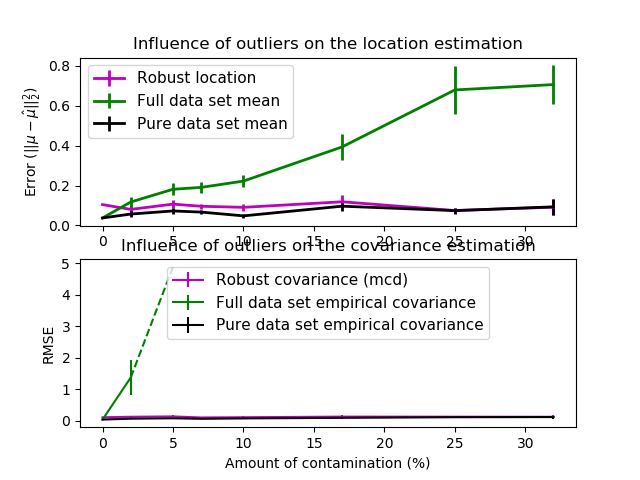
在这个例子中,我们比较了在受污染的高斯分布数据集上使用不同类型的位置估计和协方差估计时所产生的估计误差:
整个数据集的均值和经验协方差,一旦数据集中出现异常值就会分解。 稳健的MCD,它提供了一个较低的错误。 已知的好的观测值的均值和经验协方差。这可以被认为是一种“完美”的MCD估计,因此我们可以通过与这种情况进行比较来信任我们的实现。
参考
1 Johanna Hardin, David M Rocke. The distribution of robust distances. Journal of Computational and Graphical Statistics. December 1, 2005, 14(4): 928-946.
2 Zoubir A., Koivunen V., Chakhchoukh Y. and Muma M. (2012). Robust estimation in signal processing: A tutorial-style treatment of fundamental concepts. IEEE Signal Processing Magazine 29(4), 61-80.
3 P. J. Rousseeuw. Least median of squares regression. Journal of American Statistical Ass., 79:871, 1984
print(__doc__)

import numpy as np
import matplotlib.pyplot as plt
import matplotlib.font_manager

from sklearn.covariance import EmpiricalCovariance, MinCovDet

# example settings
n_samples = 80
n_features = 5
repeat = 10

range_n_outliers = np.concatenate(
    (np.linspace(0, n_samples / 8, 5),
     np.linspace(n_samples / 8, n_samples / 2, 5)[1:-1])).astype(np.int)

# definition of arrays to store results
err_loc_mcd = np.zeros((range_n_outliers.size, repeat))
err_cov_mcd = np.zeros((range_n_outliers.size, repeat))
err_loc_emp_full = np.zeros((range_n_outliers.size, repeat))
err_cov_emp_full = np.zeros((range_n_outliers.size, repeat))
err_loc_emp_pure = np.zeros((range_n_outliers.size, repeat))
err_cov_emp_pure = np.zeros((range_n_outliers.size, repeat))

# computation
for i, n_outliers in enumerate(range_n_outliers):
    for j in range(repeat):

        rng = np.random.RandomState(i * j)

        # generate data
        X = rng.randn(n_samples, n_features)
        # add some outliers
        outliers_index = rng.permutation(n_samples)[:n_outliers]
        outliers_offset = 10. * \
            (np.random.randint(2, size=(n_outliers, n_features)) - 0.5)
        X[outliers_index] += outliers_offset
        inliers_mask = np.ones(n_samples).astype(bool)
        inliers_mask[outliers_index] = False

        # fit a Minimum Covariance Determinant (MCD) robust estimator to data
        mcd = MinCovDet().fit(X)
        # compare raw robust estimates with the true location and covariance
        err_loc_mcd[i, j] = np.sum(mcd.location_ ** 2)
        err_cov_mcd[i, j] = mcd.error_norm(np.eye(n_features))

        # compare estimators learned from the full data set with true
        # parameters
        err_loc_emp_full[i, j] = np.sum(X.mean(0) ** 2)
        err_cov_emp_full[i, j] = EmpiricalCovariance().fit(X).error_norm(
            np.eye(n_features))

        # compare with an empirical covariance learned from a pure data set
        # (i.e. "perfect" mcd)
        pure_X = X[inliers_mask]
        pure_location = pure_X.mean(0)
        pure_emp_cov = EmpiricalCovariance().fit(pure_X)
        err_loc_emp_pure[i, j] = np.sum(pure_location ** 2)
        err_cov_emp_pure[i, j] = pure_emp_cov.error_norm(np.eye(n_features))

# Display results
font_prop = matplotlib.font_manager.FontProperties(size=11)
plt.subplot(2, 1, 1)
lw = 2
plt.errorbar(range_n_outliers, err_loc_mcd.mean(1),
             yerr=err_loc_mcd.std(1) / np.sqrt(repeat),
             label="Robust location", lw=lw, color='m')
plt.errorbar(range_n_outliers, err_loc_emp_full.mean(1),
             yerr=err_loc_emp_full.std(1) / np.sqrt(repeat),
             label="Full data set mean", lw=lw, color='green')
plt.errorbar(range_n_outliers, err_loc_emp_pure.mean(1),
             yerr=err_loc_emp_pure.std(1) / np.sqrt(repeat),
             label="Pure data set mean", lw=lw, color='black')
plt.title("Influence of outliers on the location estimation")
plt.ylabel(r"Error ($||\mu - \hat{\mu}||_2^2$)")
plt.legend(loc="upper left", prop=font_prop)

plt.subplot(2, 1, 2)
x_size = range_n_outliers.size
plt.errorbar(range_n_outliers, err_cov_mcd.mean(1),
             yerr=err_cov_mcd.std(1),
             label="Robust covariance (mcd)", color='m')
plt.errorbar(range_n_outliers[:(x_size // 5 + 1)],
             err_cov_emp_full.mean(1)[:(x_size // 5 + 1)],
             yerr=err_cov_emp_full.std(1)[:(x_size // 5 + 1)],
             label="Full data set empirical covariance", color='green')
plt.plot(range_n_outliers[(x_size // 5):(x_size // 2 - 1)],
         err_cov_emp_full.mean(1)[(x_size // 5):(x_size // 2 - 1)],
         color='green', ls='--')
plt.errorbar(range_n_outliers, err_cov_emp_pure.mean(1),
             yerr=err_cov_emp_pure.std(1),
             label="Pure data set empirical covariance", color='black')
plt.title("Influence of outliers on the covariance estimation")
plt.xlabel("Amount of contamination (%)")
plt.ylabel("RMSE")
plt.legend(loc="upper center", prop=font_prop)

plt.show()
脚本的总运行时间:(0分3.170秒)
Download Python source code:plot_robust_vs_empirical_covariance.py
Download Jupyter notebook:plot_robust_vs_empirical_covariance.ipynb

