

手写数字数据上K均值聚类的一个演示
在这个例子中,我们比较了K-均值的各种初始化策略在运行时和结果的质量方面。
由于这里已知的基本真相,我们还应用不同的聚类质量度量来评估聚类标签是否适合于基本的真理。
聚类质量指标评价(看 聚类行为评估对于度量的定义和讨论)。
| Shorthand | full name |
|---|---|
| homo | homogeneity score |
| compl | completeness score |
| v-meas | V measure |
| ARI | adjusted Rand index |
| AMI | adjusted mutual information |
| silhouette | silhouette coefficient |
n_digits: 10,    n_samples 1797,         n_features 64
__________________________________________________________________________________
init            time    inertia homo    compl   v-meas  ARI     AMI     silhouette
k-means++       0.24s   69510   0.610   0.657   0.633   0.481   0.629   0.129
random          0.21s   69907   0.633   0.674   0.653   0.518   0.649   0.131
PCA-based       0.02s   70768   0.668   0.695   0.681   0.558   0.678   0.142
__________________________________________________________________________________
print(__doc__)
from time import time
import numpy as np
import matplotlib.pyplot as plt
from sklearn import metrics
from sklearn.cluster import KMeans
from sklearn.datasets import load_digits
from sklearn.decomposition import PCA
from sklearn.preprocessing import scale
np.random.seed(42)
X_digits, y_digits = load_digits(return_X_y=True)
data = scale(X_digits)
n_samples, n_features = data.shape
n_digits = len(np.unique(y_digits))
labels = y_digits
sample_size = 300
print("n_digits: %d, \t n_samples %d, \t n_features %d"
% (n_digits, n_samples, n_features))
print(82 * '_')
print('init\t\ttime\tinertia\thomo\tcompl\tv-meas\tARI\tAMI\tsilhouette')
def bench_k_means(estimator, name, data):
t0 = time()
estimator.fit(data)
print('%-9s\t%.2fs\t%i\t%.3f\t%.3f\t%.3f\t%.3f\t%.3f\t%.3f'
% (name, (time() - t0), estimator.inertia_,
metrics.homogeneity_score(labels, estimator.labels_),
metrics.completeness_score(labels, estimator.labels_),
metrics.v_measure_score(labels, estimator.labels_),
metrics.adjusted_rand_score(labels, estimator.labels_),
metrics.adjusted_mutual_info_score(labels, estimator.labels_),
metrics.silhouette_score(data, estimator.labels_,
metric='euclidean',
sample_size=sample_size)))
bench_k_means(KMeans(init='k-means++', n_clusters=n_digits, n_init=10),
name="k-means++", data=data)
bench_k_means(KMeans(init='random', n_clusters=n_digits, n_init=10),
name="random", data=data)
# in this case the seeding of the centers is deterministic, hence we run the
# kmeans algorithm only once with n_init=1
pca = PCA(n_components=n_digits).fit(data)
bench_k_means(KMeans(init=pca.components_, n_clusters=n_digits, n_init=1),
name="PCA-based",
data=data)
print(82 * '_')
# #############################################################################
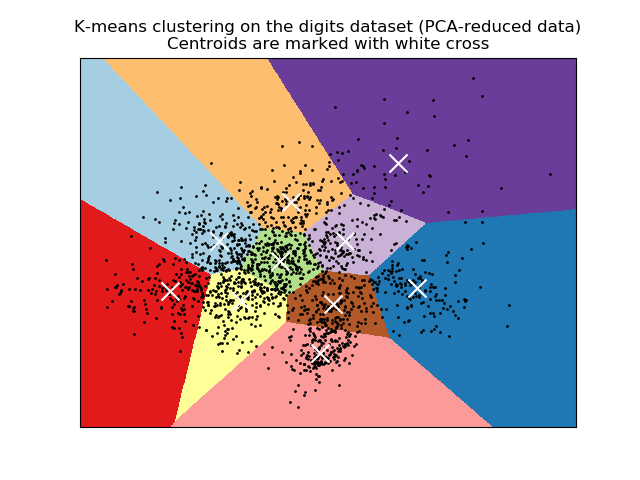
# Visualize the results on PCA-reduced data
reduced_data = PCA(n_components=2).fit_transform(data)
kmeans = KMeans(init='k-means++', n_clusters=n_digits, n_init=10)
kmeans.fit(reduced_data)
# Step size of the mesh. Decrease to increase the quality of the VQ.
h = .02 # point in the mesh [x_min, x_max]x[y_min, y_max].
# Plot the decision boundary. For that, we will assign a color to each
x_min, x_max = reduced_data[:, 0].min() - 1, reduced_data[:, 0].max() + 1
y_min, y_max = reduced_data[:, 1].min() - 1, reduced_data[:, 1].max() + 1
xx, yy = np.meshgrid(np.arange(x_min, x_max, h), np.arange(y_min, y_max, h))
# Obtain labels for each point in mesh. Use last trained model.
Z = kmeans.predict(np.c_[xx.ravel(), yy.ravel()])
# Put the result into a color plot
Z = Z.reshape(xx.shape)
plt.figure(1)
plt.clf()
plt.imshow(Z, interpolation='nearest',
extent=(xx.min(), xx.max(), yy.min(), yy.max()),
cmap=plt.cm.Paired,
aspect='auto', origin='lower')
plt.plot(reduced_data[:, 0], reduced_data[:, 1], 'k.', markersize=2)
# Plot the centroids as a white X
centroids = kmeans.cluster_centers_
plt.scatter(centroids[:, 0], centroids[:, 1],
marker='x', s=169, linewidths=3,
color='w', zorder=10)
plt.title('K-means clustering on the digits dataset (PCA-reduced data)\n'
'Centroids are marked with white cross')
plt.xlim(x_min, x_max)
plt.ylim(y_min, y_max)
plt.xticks(())
plt.yticks(())
plt.show()
脚本的总运行时间:(0分0.865秒)

