分层聚类：结构化区域与非结构化区域¶

通过示例构建一个swiss roll数据集，并在其位置上运行分层聚类。

获取更多信息， 看层次聚类

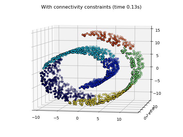
在第一步中，分层聚类是在没有结构连接约束的情况下执行的，并且只基于距离，而在第二步中，聚类被限制在k-最近邻图上：这是一种结构优先的分层聚类。

一些在没有连接约束的情况下学习到的聚类不尊重 swiss roll的结构，并且跨越流形的不同褶皱进行扩展。相反，当相反的连接约束时，聚类形成了swiss roll的一个很好的部分。

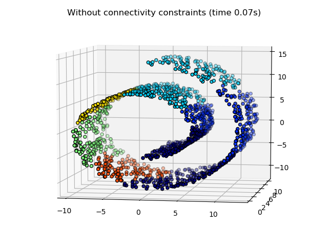
Compute unstructured hierarchical clustering...
Elapsed time: 0.07s
Number of points: 1500
Compute structured hierarchical clustering...
Elapsed time: 0.13s
Number of points: 1500

# Authors : Vincent Michel, 2010
#           Alexandre Gramfort, 2010
#           Gael Varoquaux, 2010
# License: BSD 3 clause

print(__doc__)

import time as time
import numpy as np
import matplotlib.pyplot as plt
import mpl_toolkits.mplot3d.axes3d as p3
from sklearn.cluster import AgglomerativeClustering
from sklearn.datasets import make_swiss_roll

# #############################################################################
# Generate data (swiss roll dataset)
n_samples = 1500
noise = 0.05
X, _ = make_swiss_roll(n_samples, noise=noise)
# Make it thinner
X[:, 1] *= .5

# #############################################################################
# Compute clustering
print("Compute unstructured hierarchical clustering...")
st = time.time()
ward = AgglomerativeClustering(n_clusters=6, linkage='ward').fit(X)
elapsed_time = time.time() - st
label = ward.labels_
print("Elapsed time: %.2fs" % elapsed_time)
print("Number of points: %i" % label.size)

# #############################################################################
# Plot result
fig = plt.figure()
ax = p3.Axes3D(fig)
ax.view_init(7, -80)
for l in np.unique(label):
    ax.scatter(X[label == l, 0], X[label == l, 1], X[label == l, 2],
               color=plt.cm.jet(np.float(l) / np.max(label + 1)),
               s=20, edgecolor='k')
plt.title('Without connectivity constraints (time %.2fs)' % elapsed_time)


# #############################################################################
# Define the structure A of the data. Here a 10 nearest neighbors
from sklearn.neighbors import kneighbors_graph
connectivity = kneighbors_graph(X, n_neighbors=10, include_self=False)

# #############################################################################
# Compute clustering
print("Compute structured hierarchical clustering...")
st = time.time()
ward = AgglomerativeClustering(n_clusters=6, connectivity=connectivity,
                               linkage='ward').fit(X)
elapsed_time = time.time() - st
label = ward.labels_
print("Elapsed time: %.2fs" % elapsed_time)
print("Number of points: %i" % label.size)

# #############################################################################
# Plot result
fig = plt.figure()
ax = p3.Axes3D(fig)
ax.view_init(7, -80)
for l in np.unique(label):
    ax.scatter(X[label == l, 0], X[label == l, 1], X[label == l, 2],
               color=plt.cm.jet(float(l) / np.max(label + 1)),
               s=20, edgecolor='k')
plt.title('With connectivity constraints (time %.2fs)' % elapsed_time)

plt.show()

脚本的总运行时间：(0分0.524秒)

Download Python source code:plot_ward_structured_vs_unstructured.py

Download Jupyter notebook:plot_ward_structured_vs_unstructured.ipynb