

三分类的概率校准
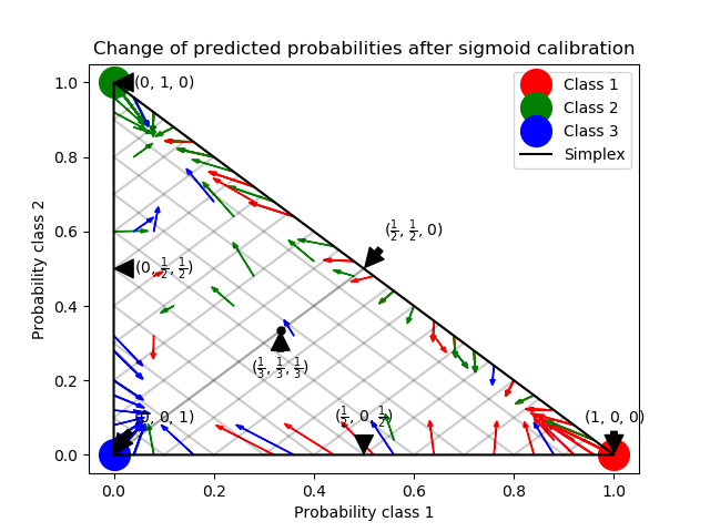
此示例说明了sigmoid如何校准三分类问题预测的概率。举例说明的是标准的2-simplex,其中三个角对应于三个类。箭头指向由未校准分类器预测的概率向量到同一分类器在hold-out 验证集上进行sigmoid校准后预测的概率向量。颜色表示实例的真正类(红色:1类,绿色:2类,蓝色:3类)。
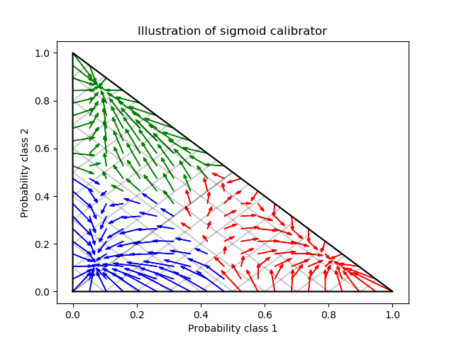
基分类器是具有25个基估计器(树)的随机林分类器。如果这个分类器对所有800个训练数据点都进行了训练,那么它对它的预测过于自信,从而导致大量的日志丢失。校准一个相同的分类器, 这个分类器在600个数据点上被训练, 在其余的200个数据点上用 method=’sigmoid’降低了预测的可信度。即, 将概率向量从simplex的边缘, 移动到中心。这种校准导致较低的对数损失。既然这种替代选择不得不增加基估计器 的数量, 这将导致类似的对数损失(log-loss)。
Log-loss of
 * uncalibrated classifier trained on 800 datapoints: 1.280
 * classifier trained on 600 datapoints and calibrated on 200 datapoint: 0.534
print(__doc__)

# Author: Jan Hendrik Metzen <jhm@informatik.uni-bremen.de>
# License: BSD Style.


import matplotlib.pyplot as plt

import numpy as np

from sklearn.datasets import make_blobs
from sklearn.ensemble import RandomForestClassifier
from sklearn.calibration import CalibratedClassifierCV
from sklearn.metrics import log_loss

np.random.seed(0)

# Generate data
X, y = make_blobs(n_samples=1000, random_state=42, cluster_std=5.0)
X_train, y_train = X[:600], y[:600]
X_valid, y_valid = X[600:800], y[600:800]
X_train_valid, y_train_valid = X[:800], y[:800]
X_test, y_test = X[800:], y[800:]

# Train uncalibrated random forest classifier on whole train and validation
# data and evaluate on test data
clf = RandomForestClassifier(n_estimators=25)
clf.fit(X_train_valid, y_train_valid)
clf_probs = clf.predict_proba(X_test)
score = log_loss(y_test, clf_probs)

# Train random forest classifier, calibrate on validation data and evaluate
# on test data
clf = RandomForestClassifier(n_estimators=25)
clf.fit(X_train, y_train)
clf_probs = clf.predict_proba(X_test)
sig_clf = CalibratedClassifierCV(clf, method="sigmoid", cv="prefit")
sig_clf.fit(X_valid, y_valid)
sig_clf_probs = sig_clf.predict_proba(X_test)
sig_score = log_loss(y_test, sig_clf_probs)

# Plot changes in predicted probabilities via arrows
plt.figure()
colors = ["r", "g", "b"]
for i in range(clf_probs.shape[0]):
    plt.arrow(clf_probs[i, 0], clf_probs[i, 1],
              sig_clf_probs[i, 0] - clf_probs[i, 0],
              sig_clf_probs[i, 1] - clf_probs[i, 1],
              color=colors[y_test[i]], head_width=1e-2)

# Plot perfect predictions
plt.plot([1.0], [0.0], 'ro', ms=20, label="Class 1")
plt.plot([0.0], [1.0], 'go', ms=20, label="Class 2")
plt.plot([0.0], [0.0], 'bo', ms=20, label="Class 3")

# Plot boundaries of unit simplex
plt.plot([0.0, 1.0, 0.0, 0.0], [0.0, 0.0, 1.0, 0.0], 'k', label="Simplex")

# Annotate points on the simplex
plt.annotate(r'($\frac{1}{3}$, $\frac{1}{3}$, $\frac{1}{3}$)',
             xy=(1.0/3, 1.0/3), xytext=(1.0/3, .23), xycoords='data',
             arrowprops=dict(facecolor='black', shrink=0.05),
             horizontalalignment='center', verticalalignment='center')
plt.plot([1.0/3], [1.0/3], 'ko', ms=5)
plt.annotate(r'($\frac{1}{2}$, $0$, $\frac{1}{2}$)',
             xy=(.5, .0), xytext=(.5, .1), xycoords='data',
             arrowprops=dict(facecolor='black', shrink=0.05),
             horizontalalignment='center', verticalalignment='center')
plt.annotate(r'($0$, $\frac{1}{2}$, $\frac{1}{2}$)',
             xy=(.0, .5), xytext=(.1, .5), xycoords='data',
             arrowprops=dict(facecolor='black', shrink=0.05),
             horizontalalignment='center', verticalalignment='center')
plt.annotate(r'($\frac{1}{2}$, $\frac{1}{2}$, $0$)',
             xy=(.5, .5), xytext=(.6, .6), xycoords='data',
             arrowprops=dict(facecolor='black', shrink=0.05),
             horizontalalignment='center', verticalalignment='center')
plt.annotate(r'($0$, $0$, $1$)',
             xy=(0, 0), xytext=(.1, .1), xycoords='data',
             arrowprops=dict(facecolor='black', shrink=0.05),
             horizontalalignment='center', verticalalignment='center')
plt.annotate(r'($1$, $0$, $0$)',
             xy=(1, 0), xytext=(1, .1), xycoords='data',
             arrowprops=dict(facecolor='black', shrink=0.05),
             horizontalalignment='center', verticalalignment='center')
plt.annotate(r'($0$, $1$, $0$)',
             xy=(0, 1), xytext=(.1, 1), xycoords='data',
             arrowprops=dict(facecolor='black', shrink=0.05),
             horizontalalignment='center', verticalalignment='center')
# Add grid
plt.grid(False)
for x in [0.0, 0.1, 0.2, 0.3, 0.4, 0.5, 0.6, 0.7, 0.8, 0.9, 1.0]:
    plt.plot([0, x], [x, 0], 'k', alpha=0.2)
    plt.plot([0, 0 + (1-x)/2], [x, x + (1-x)/2], 'k', alpha=0.2)
    plt.plot([x, x + (1-x)/2], [0, 0 + (1-x)/2], 'k', alpha=0.2)

plt.title("Change of predicted probabilities after sigmoid calibration")
plt.xlabel("Probability class 1")
plt.ylabel("Probability class 2")
plt.xlim(-0.05, 1.05)
plt.ylim(-0.05, 1.05)
plt.legend(loc="best")

print("Log-loss of")
print(" * uncalibrated classifier trained on 800 datapoints: %.3f "
      % score)
print(" * classifier trained on 600 datapoints and calibrated on "
      "200 datapoint: %.3f" % sig_score)

# Illustrate calibrator
plt.figure()
# generate grid over 2-simplex
p1d = np.linspace(0, 1, 20)
p0, p1 = np.meshgrid(p1d, p1d)
p2 = 1 - p0 - p1
p = np.c_[p0.ravel(), p1.ravel(), p2.ravel()]
p = p[p[:, 2] >= 0]

calibrated_classifier = sig_clf.calibrated_classifiers_[0]
prediction = np.vstack([calibrator.predict(this_p)
                        for calibrator, this_p in
                        zip(calibrated_classifier.calibrators_, p.T)]).T
prediction /= prediction.sum(axis=1)[:, None]

# Plot modifications of calibrator
for i in range(prediction.shape[0]):
    plt.arrow(p[i, 0], p[i, 1],
              prediction[i, 0] - p[i, 0], prediction[i, 1] - p[i, 1],
              head_width=1e-2, color=colors[np.argmax(p[i])])
# Plot boundaries of unit simplex
plt.plot([0.0, 1.0, 0.0, 0.0], [0.0, 0.0, 1.0, 0.0], 'k', label="Simplex")

plt.grid(False)
for x in [0.0, 0.1, 0.2, 0.3, 0.4, 0.5, 0.6, 0.7, 0.8, 0.9, 1.0]:
    plt.plot([0, x], [x, 0], 'k', alpha=0.2)
    plt.plot([0, 0 + (1-x)/2], [x, x + (1-x)/2], 'k', alpha=0.2)
    plt.plot([x, x + (1-x)/2], [0, 0 + (1-x)/2], 'k', alpha=0.2)

plt.title("Illustration of sigmoid calibrator")
plt.xlabel("Probability class 1")
plt.ylabel("Probability class 2")
plt.xlim(-0.05, 1.05)
plt.ylim(-0.05, 1.05)

plt.show()
脚本的总运行时间:(0分0.814秒)

