

部分依赖图
部分依赖图表示目标函数[2]与一组“目标”特征之间的依赖关系,在所有其他特征(补集特征)的值上边际化。由于人类感知能力的限制,目标特征集的大小必须很小(通常是一两个),因此目标特征通常是最重要的特征之一。
此示例演示如何从MLPRegressor和在加利福尼亚住房数据集上训练的HistGradientBoostingRegressor获取部分依赖图。这个例子取自[1]。
图显示四个 1-way 和两个单向部分依赖图(由于计算时间而被MLPRegressor省略)。单向PDP的目标变量是:中等收入(MedInc)、每户平均住户(AvgOccup)、中位住房年龄(HouseAge)和平均每户房间(AveRooms)。
1 T. Hastie, R. Tibshirani and J. Friedman, “Elements of Statistical Learning Ed. 2”, Springer, 2009.
2 For classification you can think of it as the regression score before the link function.
print(__doc__)

from time import time
import numpy as np
import pandas as pd
import matplotlib.pyplot as plt
from mpl_toolkits.mplot3d import Axes3D

from sklearn.model_selection import train_test_split
from sklearn.preprocessing import QuantileTransformer
from sklearn.pipeline import make_pipeline

from sklearn.inspection import partial_dependence
from sklearn.inspection import plot_partial_dependence
from sklearn.experimental import enable_hist_gradient_boosting  # noqa
from sklearn.ensemble import HistGradientBoostingRegressor
from sklearn.neural_network import MLPRegressor
from sklearn.datasets import fetch_california_housing
California Housing数据集预处理
避免梯度提升偏差的中心目标:使用“递归”方法的梯度提升不考虑初始估计量(这里是平均目标,默认情况下)
cal_housing = fetch_california_housing()
X = pd.DataFrame(cal_housing.data, columns=cal_housing.feature_names)
y = cal_housing.target

y -= y.mean()

X_train, X_test, y_train, y_test = train_test_split(X, y, test_size=0.1,
                                                    random_state=0)
多层感知器的局部依赖计算
让我们来拟合一个MLPRegressor,并计算单变量部分依赖图。
print("Training MLPRegressor...")
tic = time()
est = make_pipeline(QuantileTransformer(),
                    MLPRegressor(hidden_layer_sizes=(50, 50),
                                 learning_rate_init=0.01,
                                 early_stopping=True))
est.fit(X_train, y_train)
print("done in {:.3f}s".format(time() - tic))
print("Test R2 score: {:.2f}".format(est.score(X_test, y_test)))
Training MLPRegressor...
done in 5.430s
Test R2 score: 0.81
我们配置了一条工作流来扩展数值输入特征,并调整了神经网络的大小和学习速率,从而在测试集上得到了训练时间和预测性能之间的合理折衷。
重要的是,这个表格数据集因其特征而具有非常不同的动态范围。神经网络往往对不同尺度的特征非常敏感,而忽略了对数字特征的预处理,会导致一个非常糟糕的模型。
使用更大的神经网络可以获得更高的预测性能,但训练成本也要高得多。
请注意,在绘制部分依赖之前,在测试集中检查模型是否足够准确是很重要的,因为在解释给定特征对糟糕模型的预测功能的影响方面几乎没有用处。
现在让我们使用模型不可知论(蛮力)方法计算这个神经网络的部分依赖图:
print('Computing partial dependence plots...')
tic = time()
# We don't compute the 2-way PDP (5, 1) here, because it is a lot slower
# with the brute method.
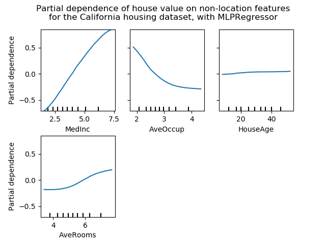
features = ['MedInc', 'AveOccup', 'HouseAge', 'AveRooms']
plot_partial_dependence(est, X_train, features,
n_jobs=3, grid_resolution=20)
print("done in {:.3f}s".format(time() - tic))
fig = plt.gcf()
fig.suptitle('Partial dependence of house value on non-location features\n'
'for the California housing dataset, with MLPRegressor')
fig.subplots_adjust(hspace=0.3)
Computing partial dependence plots...
done in 3.392s
梯度提升的部分依赖计算
现在,我们来拟合一个GradientBoostingRegressor,计算部分依赖图,或者一次计算一个或两个变量。
print("Training GradientBoostingRegressor...")
tic = time()
est = HistGradientBoostingRegressor()
est.fit(X_train, y_train)
print("done in {:.3f}s".format(time() - tic))
print("Test R2 score: {:.2f}".format(est.score(X_test, y_test)))
Training GradientBoostingRegressor...
done in 0.757s
Test R2 score: 0.85
在这里,我们使用了梯度提升模型的默认超参数,而无需进行任何预处理,因为基于树的模型对数值特征的单调变换具有很强的鲁棒性。
请注意,在这个表格数据集上,梯度提升机的训练速度和精度都比神经网络快得多。调优它们的超参数也要便宜得多(默认参数往往运行良好,而神经网络通常不是这样)。
最后,正如我们接下来将看到的那样,基于部分依赖图树的模型计算速度也快了几个数量级,这使得为一对交互特征计算部分依赖图的成本更低:
print('Computing partial dependence plots...')
tic = time()
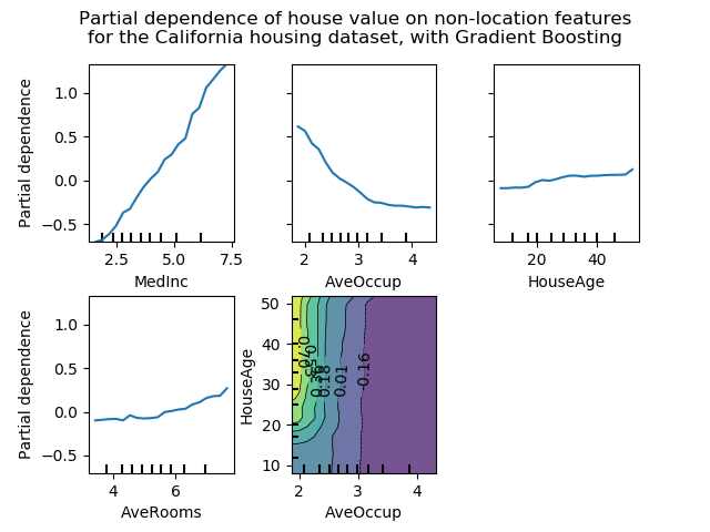
features = ['MedInc', 'AveOccup', 'HouseAge', 'AveRooms',
('AveOccup', 'HouseAge')]
plot_partial_dependence(est, X_train, features,
n_jobs=3, grid_resolution=20)
print("done in {:.3f}s".format(time() - tic))
fig = plt.gcf()
fig.suptitle('Partial dependence of house value on non-location features\n'
'for the California housing dataset, with Gradient Boosting')
fig.subplots_adjust(wspace=0.4, hspace=0.3)
Computing partial dependence plots...
done in 0.230s
图分析
我们可以清楚地看到,中位房价与收入中位数(左上角)呈线性关系,当每个家庭的平均居住者增加(上、中)时,房价下降。右上角的显示,一个地区的房屋年龄对房价(中位数)没有很大的影响;每户平均房数也是如此。x轴上的勾标表示训练数据中特征值的十进制。
我们还观察到 MLPRegressor比组HistGradientBoostingRegressor有更好的预测。为了使这些图具有可比性,有必要减去目标y的平均值:默认情况下,用于组HistGradientBoostingRegressor的“递归”方法不考虑初始预测器(在本例中为平均目标)。将目标平均值设置为0可以避免这种偏差。
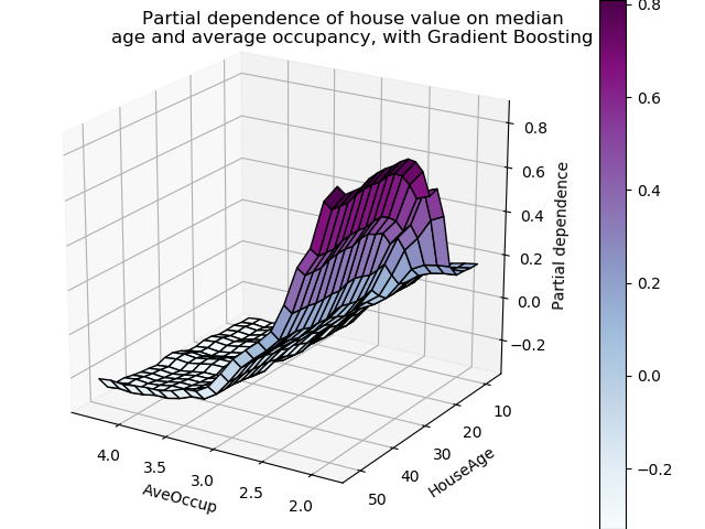
具有两个目标特征的局部依赖图使我们能够可视化它们之间的交互作用。双向部分依赖图显示了住宅价格中位数与住房年龄和平均居住者的共同值之间的相关性。我们可以清楚地看到这两种特征之间的相互作用:对于平均入住率大于2的情况,房价几乎与住房年龄无关,而对于小于2的价值,则对年龄有很强的依赖性。
三维交互图
让我们为这两个特性的交互绘制同样的部分依赖图,这一次是在三维中。
fig = plt.figure()

features = ('AveOccup', 'HouseAge')
pdp, axes = partial_dependence(est, X_train, features=features,
                               grid_resolution=20)
XX, YY = np.meshgrid(axes[0], axes[1])
Z = pdp[0].T
ax = Axes3D(fig)
surf = ax.plot_surface(XX, YY, Z, rstride=1, cstride=1,
                       cmap=plt.cm.BuPu, edgecolor='k')
ax.set_xlabel(features[0])
ax.set_ylabel(features[1])
ax.set_zlabel('Partial dependence')
#  pretty init view
ax.view_init(elev=22, azim=122)
plt.colorbar(surf)
plt.suptitle('Partial dependence of house value on median\n'
             'age and average occupancy, with Gradient Boosting')
plt.subplots_adjust(top=0.9)

plt.show()
 脚本的总运行时间:(0分11.818秒)

