

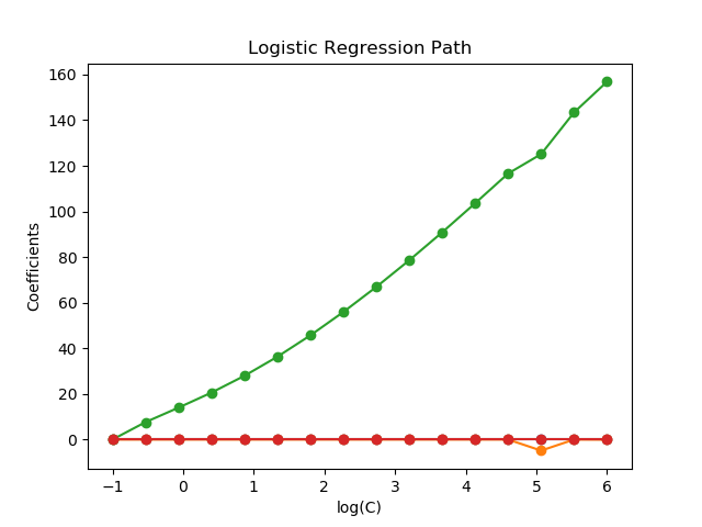
L1-Logistic回归的正则化路径
基于iris数据集的二分类问题训练 L1-惩罚 Logistic回归模型。
模型由强正则化到最少正则化。模型的4个系数被收集并绘制成“正则化路径”:在图的左边(强正则化者),所有系数都精确地为0。当正则化逐步放松时,系数可以一个接一个地得到非零值。
在这里,我们选择了线性求解器,因为它可以有效地优化非光滑的、稀疏的带l1惩罚的Logistic回归损失。
还请注意,我们为公差设置了一个较低的值,以确保模型在收集系数之前已经收敛。
Computing regularization path ...
This took 0.072s
print(__doc__)

# Author: Alexandre Gramfort <alexandre.gramfort@inria.fr>
# License: BSD 3 clause

from time import time
import numpy as np
import matplotlib.pyplot as plt

from sklearn import linear_model
from sklearn import datasets
from sklearn.svm import l1_min_c

iris = datasets.load_iris()
X = iris.data
y = iris.target

X = X[y != 2]
y = y[y != 2]

X /= X.max()  # Normalize X to speed-up convergence

# #############################################################################
# Demo path functions

cs = l1_min_c(X, y, loss='log') * np.logspace(0, 7, 16)


print("Computing regularization path ...")
start = time()
clf = linear_model.LogisticRegression(penalty='l1', solver='liblinear',
                                      tol=1e-6, max_iter=int(1e6),
                                      warm_start=True,
                                      intercept_scaling=10000.)
coefs_ = []
for c in cs:
    clf.set_params(C=c)
    clf.fit(X, y)
    coefs_.append(clf.coef_.ravel().copy())
print("This took %0.3fs" % (time() - start))

coefs_ = np.array(coefs_)
plt.plot(np.log10(cs), coefs_, marker='o')
ymin, ymax = plt.ylim()
plt.xlabel('log(C)')
plt.ylabel('Coefficients')
plt.title('Logistic Regression Path')
plt.axis('tight')
plt.show()
脚本的总运行时间:(0分0.151秒)

