基于完全随机树的哈希特征变换¶

RandomTreesEmbedding 提供了一种将数据映射到非常高维、稀疏表示的方法，这可能有利于分类。该映射是完全无监督和非常有效的。

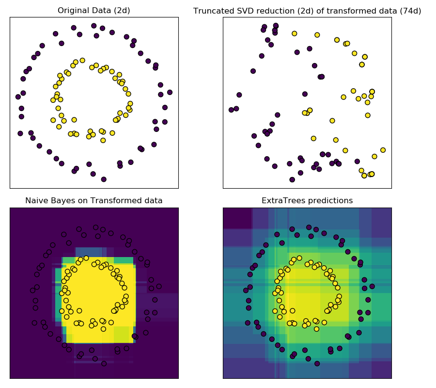
这个例子可视化了由几个树给出的分区，并展示了转换也可以用于非线性维数约简或非线性分类。

相邻的点通常共享一棵树的同一片叶子，因此他们的哈希表示共享一个大区域。这样就可以将两个同心圆简单分离， 主要是基于转换后数据的主成分， 使用带约束的SVD。

在高维空间中，线性分类器往往具有很好的精度。对于稀疏二进制数据，bernoulliNB特别适合。下面一行将比较从BernoulliNB在转换后数据集上训练得到的决策边界与使用极端随机树森林在原始数据集上训练得到的决策边界进行比较。

import numpy as np
import matplotlib.pyplot as plt

from sklearn.datasets import make_circles
from sklearn.ensemble import RandomTreesEmbedding, ExtraTreesClassifier
from sklearn.decomposition import TruncatedSVD
from sklearn.naive_bayes import BernoulliNB

# make a synthetic dataset
X, y = make_circles(factor=0.5, random_state=0, noise=0.05)

# use RandomTreesEmbedding to transform data
hasher = RandomTreesEmbedding(n_estimators=10, random_state=0, max_depth=3)
X_transformed = hasher.fit_transform(X)

# Visualize result after dimensionality reduction using truncated SVD
svd = TruncatedSVD(n_components=2)
X_reduced = svd.fit_transform(X_transformed)

# Learn a Naive Bayes classifier on the transformed data
nb = BernoulliNB()
nb.fit(X_transformed, y)


# Learn an ExtraTreesClassifier for comparison
trees = ExtraTreesClassifier(max_depth=3, n_estimators=10, random_state=0)
trees.fit(X, y)


# scatter plot of original and reduced data
fig = plt.figure(figsize=(9, 8))

ax = plt.subplot(221)
ax.scatter(X[:, 0], X[:, 1], c=y, s=50, edgecolor='k')
ax.set_title("Original Data (2d)")
ax.set_xticks(())
ax.set_yticks(())

ax = plt.subplot(222)
ax.scatter(X_reduced[:, 0], X_reduced[:, 1], c=y, s=50, edgecolor='k')
ax.set_title("Truncated SVD reduction (2d) of transformed data (%dd)" %
             X_transformed.shape[1])
ax.set_xticks(())
ax.set_yticks(())

# Plot the decision in original space. For that, we will assign a color
# to each point in the mesh [x_min, x_max]x[y_min, y_max].
h = .01
x_min, x_max = X[:, 0].min() - .5, X[:, 0].max() + .5
y_min, y_max = X[:, 1].min() - .5, X[:, 1].max() + .5
xx, yy = np.meshgrid(np.arange(x_min, x_max, h), np.arange(y_min, y_max, h))

# transform grid using RandomTreesEmbedding
transformed_grid = hasher.transform(np.c_[xx.ravel(), yy.ravel()])
y_grid_pred = nb.predict_proba(transformed_grid)[:, 1]

ax = plt.subplot(223)
ax.set_title("Naive Bayes on Transformed data")
ax.pcolormesh(xx, yy, y_grid_pred.reshape(xx.shape))
ax.scatter(X[:, 0], X[:, 1], c=y, s=50, edgecolor='k')
ax.set_ylim(-1.4, 1.4)
ax.set_xlim(-1.4, 1.4)
ax.set_xticks(())
ax.set_yticks(())

# transform grid using ExtraTreesClassifier
y_grid_pred = trees.predict_proba(np.c_[xx.ravel(), yy.ravel()])[:, 1]

ax = plt.subplot(224)
ax.set_title("ExtraTrees predictions")
ax.pcolormesh(xx, yy, y_grid_pred.reshape(xx.shape))
ax.scatter(X[:, 0], X[:, 1], c=y, s=50, edgecolor='k')
ax.set_ylim(-1.4, 1.4)
ax.set_xlim(-1.4, 1.4)
ax.set_xticks(())
ax.set_yticks(())

plt.tight_layout()
plt.show()

脚本的总运行时间：(0分0.437秒)

Download Python source code: plot_random_forest_embedding.py

Download Jupyter notebook:plot_random_forest_embedding.ipynb