分类器校准的比较¶

举例说明分类器预测概率的校准。

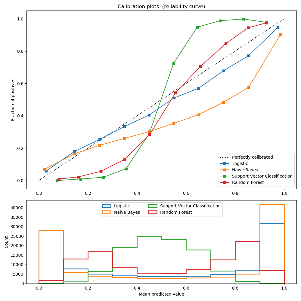
经过良好校准的分类器是概率分类器，它的输出可以直接解释为置信度。例如，经过良好校准的二分类器应该对样本进行分类，这个样本被给予的predict_proba值接近0.8，就意味着大约80%的把握属于正类。

逻辑回归返回良好的校准预测，因为它直接优化对数损失。相反，其他方法返回有偏概率，每种方法有不同的偏差：

GaussianNaiveBayes倾向于将概率推到0或1(注意直方图中的计数)。这主要是因为它假设在给定类的情况下，特征是有条件独立的，而在包含2个冗余特征的数据集中则不是这样。
随机森林分类器显示相反的行为：直方图显示接近峰值。0.2和0.9的概率，而概率接近0或1是非常罕见的。Nculescu-Mizil和Caruana [1]给出了对此的解释：“装袋和随机森林等方法--从一组基本模型的平均预测做出的预测接近0和1是很难的，因为底层基本模型中的方差会导致预测偏差，这些预测值本应该是0或者1，但是却偏离了这些值。由于预测仅限于区间[0，1]，由方差引起的误差往往是近0和1的单边误差。例如，如果一个模型应该对一个情况预测p=0，那么bagging法可以实现的唯一方法就是所有bagging中的树都预测为零。如果将噪声加到bagging中的树木上，这种噪声会导致一些树预测值大于0，从而使bagging集合的平均预测值从0偏离。我们在随机森林中观察到的这种影响最强烈，因为使用随机森林训练的基层树由于特征子集而具有较高的方差。“结果表明，校准曲线呈现出sigmoid形状，表明分类器可以更多地信任它的“直觉”，并返回接近0或1的典型概率。
支持向量分类(SVC)显示了一个比随机森林分类器更加sigmoid形状的曲线，这是典型的最大化间隔方法(比较Nculescu-Mizil和Caruana [1])，重点是关注那些接近决策边界的硬样本(支持向量)。

参考

1(1,2) Predicting Good Probabilities with Supervised Learning, A. Niculescu-Mizil & R. Caruana, ICML 2005

print(__doc__)

# Author: Jan Hendrik Metzen <jhm@informatik.uni-bremen.de>
# License: BSD Style.

import numpy as np
np.random.seed(0)

import matplotlib.pyplot as plt

from sklearn import datasets
from sklearn.naive_bayes import GaussianNB
from sklearn.linear_model import LogisticRegression
from sklearn.ensemble import RandomForestClassifier
from sklearn.svm import LinearSVC
from sklearn.calibration import calibration_curve

X, y = datasets.make_classification(n_samples=100000, n_features=20,
                                    n_informative=2, n_redundant=2)

train_samples = 100  # Samples used for training the models

X_train = X[:train_samples]
X_test = X[train_samples:]
y_train = y[:train_samples]
y_test = y[train_samples:]

# Create classifiers
lr = LogisticRegression()
gnb = GaussianNB()
svc = LinearSVC(C=1.0)
rfc = RandomForestClassifier()


# #############################################################################
# Plot calibration plots

plt.figure(figsize=(10, 10))
ax1 = plt.subplot2grid((3, 1), (0, 0), rowspan=2)
ax2 = plt.subplot2grid((3, 1), (2, 0))

ax1.plot([0, 1], [0, 1], "k:", label="Perfectly calibrated")
for clf, name in [(lr, 'Logistic'),
                  (gnb, 'Naive Bayes'),
                  (svc, 'Support Vector Classification'),
                  (rfc, 'Random Forest')]:
    clf.fit(X_train, y_train)
    if hasattr(clf, "predict_proba"):
        prob_pos = clf.predict_proba(X_test)[:, 1]
    else:  # use decision function
        prob_pos = clf.decision_function(X_test)
        prob_pos = \
            (prob_pos - prob_pos.min()) / (prob_pos.max() - prob_pos.min())
    fraction_of_positives, mean_predicted_value = \
        calibration_curve(y_test, prob_pos, n_bins=10)

    ax1.plot(mean_predicted_value, fraction_of_positives, "s-",
             label="%s" % (name, ))

    ax2.hist(prob_pos, range=(0, 1), bins=10, label=name,
             histtype="step", lw=2)

ax1.set_ylabel("Fraction of positives")
ax1.set_ylim([-0.05, 1.05])
ax1.legend(loc="lower right")
ax1.set_title('Calibration plots  (reliability curve)')

ax2.set_xlabel("Mean predicted value")
ax2.set_ylabel("Count")
ax2.legend(loc="upper center", ncol=2)

plt.tight_layout()
plt.show()

脚本的总运行时间：(0分1.370秒)