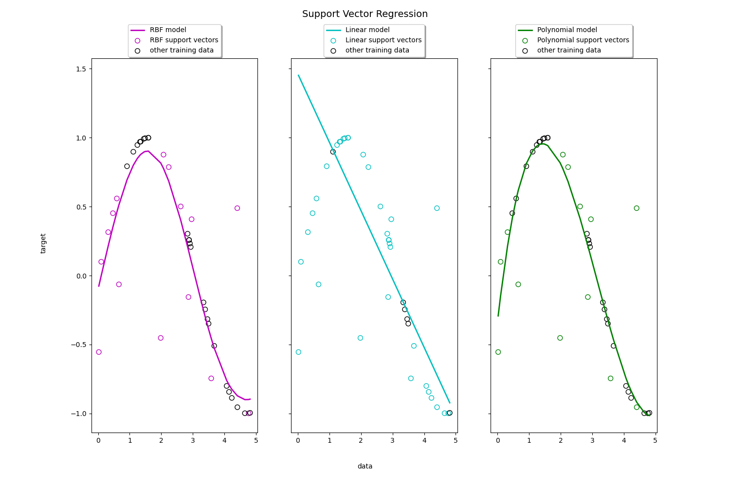
使用线性与非线性核的支持向量机回归¶

在本案例中，我们在玩具数据集上用线性、多项式及RBF核的支持向量机分别进行一维回归。

print(__doc__)

import numpy as np
from sklearn.svm import SVR
import matplotlib.pyplot as plt

# #############################################################################
# 获得样本数据
X = np.sort(5 * np.random.rand(40, 1), axis=0)
y = np.sin(X).ravel()

# #############################################################################
# 在标签中增加噪音
y[::5] += 3 * (0.5 - np.random.rand(8))

# #############################################################################
# 拟合回归模型
svr_rbf = SVR(kernel='rbf', C=100, gamma=0.1, epsilon=.1)
svr_lin = SVR(kernel='linear', C=100, gamma='auto')
svr_poly = SVR(kernel='poly', C=100, gamma='auto', degree=3, epsilon=.1,
               coef0=1)

# #############################################################################
# 查看结果
lw = 2

svrs = [svr_rbf, svr_lin, svr_poly]
kernel_label = ['RBF', 'Linear', 'Polynomial']
model_color = ['m', 'c', 'g']

fig, axes = plt.subplots(nrows=1, ncols=3, figsize=(15, 10), sharey=True)
for ix, svr in enumerate(svrs):
    axes[ix].plot(X, svr.fit(X, y).predict(X), color=model_color[ix], lw=lw,
                  label='{} model'.format(kernel_label[ix]))
    axes[ix].scatter(X[svr.support_], y[svr.support_], facecolor="none",
                     edgecolor=model_color[ix], s=50,
                     label='{} support vectors'.format(kernel_label[ix]))
    axes[ix].scatter(X[np.setdiff1d(np.arange(len(X)), svr.support_)],
                     y[np.setdiff1d(np.arange(len(X)), svr.support_)],
                     facecolor="none", edgecolor="k", s=50,
                     label='other training data')
    axes[ix].legend(loc='upper center', bbox_to_anchor=(0.5, 1.1),
                    ncol=1, fancybox=True, shadow=True)

fig.text(0.5, 0.04, 'data', ha='center', va='center')
fig.text(0.06, 0.5, 'target', ha='center', va='center', rotation='vertical')
fig.suptitle("Support Vector Regression", fontsize=14)
plt.show()

脚本的总运行时间：（0分钟4.616秒）