交叉分解法比较¶

注意 单击此处下载完整的示例代码，或通过Binder在浏览器中运行此示例

简单使用各种交叉分解算法： PLSCanonical - PLSRegression， 多变量响应， PLS2 - PLSRegression单变量响应， PLS1 - CCA。

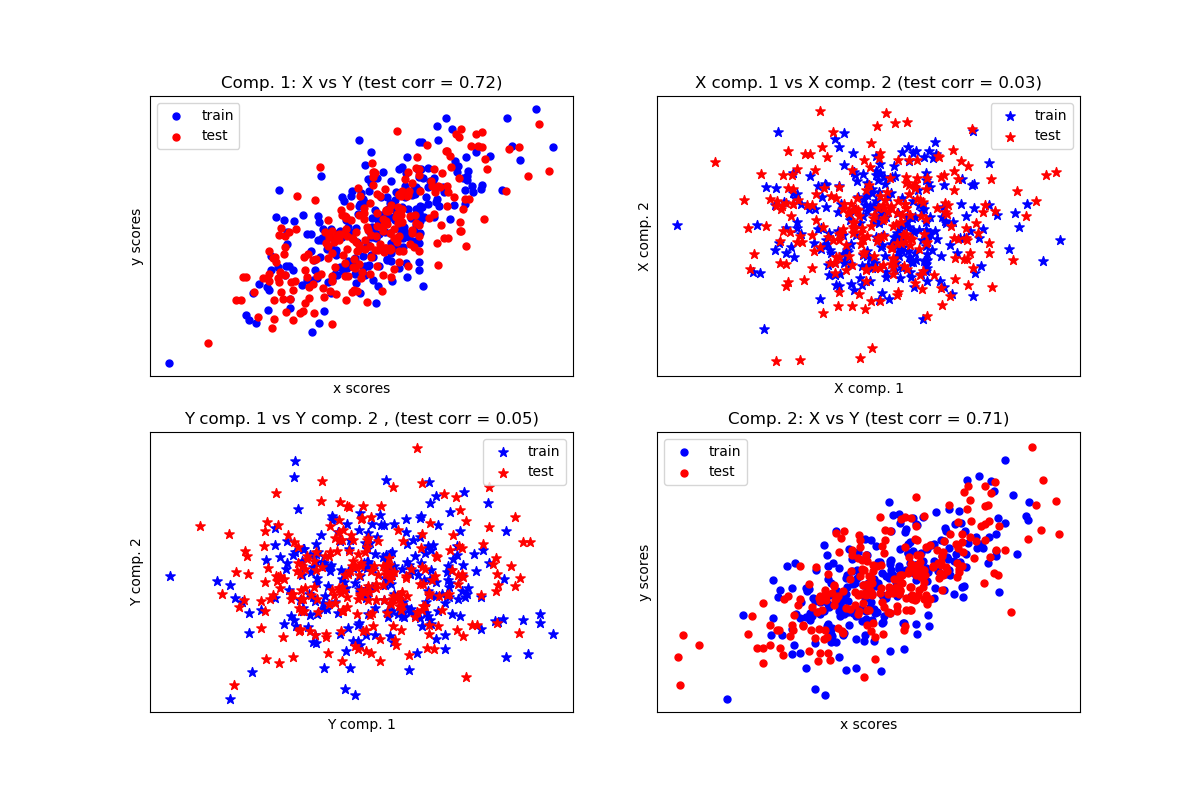
给定两个多元共变二维数据集X和Y，PLS提取协方差方向，即解释两个数据集之间最大共享方差的每个数据集的分量。这一点在散点矩阵图中有展示， 数据集X和数据集Y中的成分1是最大相关(点位于第一对角线周围)。这对于两个数据集中的成分2也是如此，但是，不同组件的数据集之间的相关性很弱：点云是非球面的。

Corr(X)
[[ 1.    0.51  0.07 -0.05]
 [ 0.51  1.    0.11 -0.01]
 [ 0.07  0.11  1.    0.49]
 [-0.05 -0.01  0.49  1.  ]]
Corr(Y)
[[1.   0.48 0.05 0.03]
 [0.48 1.   0.04 0.12]
 [0.05 0.04 1.   0.51]
 [0.03 0.12 0.51 1.  ]]
True B (such that: Y = XB + Err)
[[1 1 1]
 [2 2 2]
 [0 0 0]
 [0 0 0]
 [0 0 0]
 [0 0 0]
 [0 0 0]
 [0 0 0]
 [0 0 0]
 [0 0 0]]
Estimated B
[[ 1.   1.   1. ]
 [ 2.   2.   2. ]
 [-0.  -0.   0. ]
 [ 0.   0.   0. ]
 [ 0.   0.   0. ]
 [ 0.   0.  -0. ]
 [-0.  -0.  -0.1]
 [-0.  -0.   0. ]
 [ 0.   0.   0.1]
 [ 0.   0.  -0. ]]
Estimated betas
[[ 1. ]
 [ 2.1]
 [ 0. ]
 [ 0. ]
 [ 0. ]
 [-0. ]
 [-0. ]
 [ 0. ]
 [-0. ]
 [-0. ]]

print(__doc__)

import numpy as np
import matplotlib.pyplot as plt
from sklearn.cross_decomposition import PLSCanonical, PLSRegression, CCA

# #############################################################################
# Dataset based latent variables model

n = 500
# 2 latents vars:
l1 = np.random.normal(size=n)
l2 = np.random.normal(size=n)

latents = np.array([l1, l1, l2, l2]).T
X = latents + np.random.normal(size=4 * n).reshape((n, 4))
Y = latents + np.random.normal(size=4 * n).reshape((n, 4))

X_train = X[:n // 2]
Y_train = Y[:n // 2]
X_test = X[n // 2:]
Y_test = Y[n // 2:]

print("Corr(X)")
print(np.round(np.corrcoef(X.T), 2))
print("Corr(Y)")
print(np.round(np.corrcoef(Y.T), 2))

# #############################################################################
# Canonical (symmetric) PLS

# Transform data
# ~~~~~~~~~~~~~~
plsca = PLSCanonical(n_components=2)
plsca.fit(X_train, Y_train)
X_train_r, Y_train_r = plsca.transform(X_train, Y_train)
X_test_r, Y_test_r = plsca.transform(X_test, Y_test)

# Scatter plot of scores
# ~~~~~~~~~~~~~~~~~~~~~~
# 1) On diagonal plot X vs Y scores on each components
plt.figure(figsize=(12, 8))
plt.subplot(221)
plt.scatter(X_train_r[:, 0], Y_train_r[:, 0], label="train",
            marker="o", c="b", s=25)
plt.scatter(X_test_r[:, 0], Y_test_r[:, 0], label="test",
            marker="o", c="r", s=25)
plt.xlabel("x scores")
plt.ylabel("y scores")
plt.title('Comp. 1: X vs Y (test corr = %.2f)' %
          np.corrcoef(X_test_r[:, 0], Y_test_r[:, 0])[0, 1])
plt.xticks(())
plt.yticks(())
plt.legend(loc="best")

plt.subplot(224)
plt.scatter(X_train_r[:, 1], Y_train_r[:, 1], label="train",
            marker="o", c="b", s=25)
plt.scatter(X_test_r[:, 1], Y_test_r[:, 1], label="test",
            marker="o", c="r", s=25)
plt.xlabel("x scores")
plt.ylabel("y scores")
plt.title('Comp. 2: X vs Y (test corr = %.2f)' %
          np.corrcoef(X_test_r[:, 1], Y_test_r[:, 1])[0, 1])
plt.xticks(())
plt.yticks(())
plt.legend(loc="best")

# 2) Off diagonal plot components 1 vs 2 for X and Y
plt.subplot(222)
plt.scatter(X_train_r[:, 0], X_train_r[:, 1], label="train",
            marker="*", c="b", s=50)
plt.scatter(X_test_r[:, 0], X_test_r[:, 1], label="test",
            marker="*", c="r", s=50)
plt.xlabel("X comp. 1")
plt.ylabel("X comp. 2")
plt.title('X comp. 1 vs X comp. 2 (test corr = %.2f)'
          % np.corrcoef(X_test_r[:, 0], X_test_r[:, 1])[0, 1])
plt.legend(loc="best")
plt.xticks(())
plt.yticks(())

plt.subplot(223)
plt.scatter(Y_train_r[:, 0], Y_train_r[:, 1], label="train",
            marker="*", c="b", s=50)
plt.scatter(Y_test_r[:, 0], Y_test_r[:, 1], label="test",
            marker="*", c="r", s=50)
plt.xlabel("Y comp. 1")
plt.ylabel("Y comp. 2")
plt.title('Y comp. 1 vs Y comp. 2 , (test corr = %.2f)'
          % np.corrcoef(Y_test_r[:, 0], Y_test_r[:, 1])[0, 1])
plt.legend(loc="best")
plt.xticks(())
plt.yticks(())
plt.show()

# #############################################################################
# PLS regression, with multivariate response, a.k.a. PLS2

n = 1000
q = 3
p = 10
X = np.random.normal(size=n * p).reshape((n, p))
B = np.array([[1, 2] + [0] * (p - 2)] * q).T
# each Yj = 1*X1 + 2*X2 + noize
Y = np.dot(X, B) + np.random.normal(size=n * q).reshape((n, q)) + 5

pls2 = PLSRegression(n_components=3)
pls2.fit(X, Y)
print("True B (such that: Y = XB + Err)")
print(B)
# compare pls2.coef_ with B
print("Estimated B")
print(np.round(pls2.coef_, 1))
pls2.predict(X)

# PLS regression, with univariate response, a.k.a. PLS1

n = 1000
p = 10
X = np.random.normal(size=n * p).reshape((n, p))
y = X[:, 0] + 2 * X[:, 1] + np.random.normal(size=n * 1) + 5
pls1 = PLSRegression(n_components=3)
pls1.fit(X, y)
# note that the number of components exceeds 1 (the dimension of y)
print("Estimated betas")
print(np.round(pls1.coef_, 1))

# #############################################################################
# CCA (PLS mode B with symmetric deflation)

cca = CCA(n_components=2)
cca.fit(X_train, Y_train)
X_train_r, Y_train_r = cca.transform(X_train, Y_train)
X_test_r, Y_test_r = cca.transform(X_test, Y_test)

脚本的总运行时间：(0分0.237秒)

Download Python source code: plot_compare_cross_decomposition.py

Download Jupyter notebook: plot_compare_cross_decomposition.ipynb