

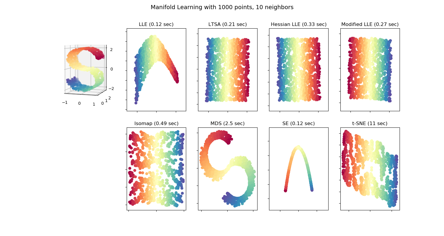
流形学习方法的比较
用多种流形学习方法对S曲线数据集降维的实例。
有关这些算法的讨论和比较,请参见manifold module page。
对于类似的示例,即将方法应用于球面数据集,参见割球面上的流形学习方法。
请注意,MDS的目的是找到数据的低维表示(这里是2D),其中距离很好地表示了原始高维空间中的距离,与其他流形学习算法不同,它不寻求低维空间中数据的各向同性表示。
/home/circleci/project/sklearn/utils/validation.py:68: FutureWarning: Pass n_neighbors=10, n_components=2 as keyword args. From version 0.25 passing these as positional arguments will result in an error
  warnings.warn("Pass {} as keyword args. From version 0.25 "
LLE: 0.12 sec
LTSA: 0.21 sec
Hessian LLE: 0.33 sec
Modified LLE: 0.27 sec
Isomap: 0.49 sec
MDS: 2.5 sec
SE: 0.12 sec
t-SNE: 11 sec
# Author: Jake Vanderplas -- <vanderplas@astro.washington.edu>

print(__doc__)

from collections import OrderedDict
from functools import partial
from time import time

import matplotlib.pyplot as plt
from mpl_toolkits.mplot3d import Axes3D
from matplotlib.ticker import NullFormatter

from sklearn import manifold, datasets

# Next line to silence pyflakes. This import is needed.
Axes3D

n_points = 1000
X, color = datasets.make_s_curve(n_points, random_state=0)
n_neighbors = 10
n_components = 2

# Create figure
fig = plt.figure(figsize=(15, 8))
fig.suptitle("Manifold Learning with %i points, %i neighbors"
             % (1000, n_neighbors), fontsize=14)

# Add 3d scatter plot
ax = fig.add_subplot(251, projection='3d')
ax.scatter(X[:, 0], X[:, 1], X[:, 2], c=color, cmap=plt.cm.Spectral)
ax.view_init(4, -72)

# Set-up manifold methods
LLE = partial(manifold.LocallyLinearEmbedding,
              n_neighbors, n_components, eigen_solver='auto')

methods = OrderedDict()
methods['LLE'] = LLE(method='standard')
methods['LTSA'] = LLE(method='ltsa')
methods['Hessian LLE'] = LLE(method='hessian')
methods['Modified LLE'] = LLE(method='modified')
methods['Isomap'] = manifold.Isomap(n_neighbors, n_components)
methods['MDS'] = manifold.MDS(n_components, max_iter=100, n_init=1)
methods['SE'] = manifold.SpectralEmbedding(n_components=n_components,
                                           n_neighbors=n_neighbors)
methods['t-SNE'] = manifold.TSNE(n_components=n_components, init='pca',
                                 random_state=0)

# Plot results
for i, (label, method) in enumerate(methods.items()):
    t0 = time()
    Y = method.fit_transform(X)
    t1 = time()
    print("%s: %.2g sec" % (label, t1 - t0))
    ax = fig.add_subplot(2, 5, 2 + i + (i > 3))
    ax.scatter(Y[:, 0], Y[:, 1], c=color, cmap=plt.cm.Spectral)
    ax.set_title("%s (%.2g sec)" % (label, t1 - t0))
    ax.xaxis.set_major_formatter(NullFormatter())
    ax.yaxis.set_major_formatter(NullFormatter())
    ax.axis('tight')

plt.show()
脚本的总运行时间:(0分15.437秒)

