

变体贝叶斯高斯混合的聚集优先类型分析
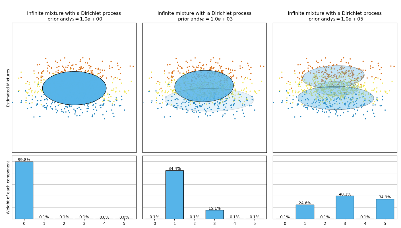
这个例子绘制了一个从toy数据集(混合了三个高斯)得到的椭球, 这些椭球是由带有Dirichlet分布先验的 (weight_concentration_prior_type='dirichlet_distribution') 和一个Dirichlet过程先验(weight_concentration_prior_type='dirichlet_process')的 BayesianGaussianMixture 类模型拟合得到的。
BayesianGaussianMixture类可以自动调整混合成分的个数。参数 weight_concentration_prior 与产生的具有非零权重的成分数有直接联系。指定聚集先验的低值将使模型将大部分权重放在少数成分上,其余成分的权重将非常接近于零。较高的聚集先验,将允许更多的成分在混合中更活跃。
Dirichlet过程先验允许定义无穷多个成分,并自动选择正确的成分的个数:它只在必要时激活成分。
相反,具有Dirichlet分布先验的经典有限混合模型更倾向于更均匀的权重成分,因此,它倾向于将自然聚类划分为不必要的子成分。

# Author: Thierry Guillemot <thierry.guillemot.work@gmail.com>
# License: BSD 3 clause

import numpy as np
import matplotlib as mpl
import matplotlib.pyplot as plt
import matplotlib.gridspec as gridspec

from sklearn.mixture import BayesianGaussianMixture

print(__doc__)


def plot_ellipses(ax, weights, means, covars):
    for n in range(means.shape[0]):
        eig_vals, eig_vecs = np.linalg.eigh(covars[n])
        unit_eig_vec = eig_vecs[0] / np.linalg.norm(eig_vecs[0])
        angle = np.arctan2(unit_eig_vec[1], unit_eig_vec[0])
        # Ellipse needs degrees
        angle = 180 * angle / np.pi
        # eigenvector normalization
        eig_vals = 2 * np.sqrt(2) * np.sqrt(eig_vals)
        ell = mpl.patches.Ellipse(means[n], eig_vals[0], eig_vals[1],
                                  180 + angle, edgecolor='black')
        ell.set_clip_box(ax.bbox)
        ell.set_alpha(weights[n])
        ell.set_facecolor('#56B4E9')
        ax.add_artist(ell)


def plot_results(ax1, ax2, estimator, X, y, title, plot_title=False):
    ax1.set_title(title)
    ax1.scatter(X[:, 0], X[:, 1], s=5, marker='o', color=colors[y], alpha=0.8)
    ax1.set_xlim(-2., 2.)
    ax1.set_ylim(-3., 3.)
    ax1.set_xticks(())
    ax1.set_yticks(())
    plot_ellipses(ax1, estimator.weights_, estimator.means_,
                  estimator.covariances_)

    ax2.get_xaxis().set_tick_params(direction='out')
    ax2.yaxis.grid(True, alpha=0.7)
    for k, w in enumerate(estimator.weights_):
        ax2.bar(k, w, width=0.9, color='#56B4E9', zorder=3,
                align='center', edgecolor='black')
        ax2.text(k, w + 0.007, "%.1f%%" % (w * 100.),
                 horizontalalignment='center')
    ax2.set_xlim(-.6, 2 * n_components - .4)
    ax2.set_ylim(0., 1.1)
    ax2.tick_params(axis='y', which='both', left=False,
                    right=False, labelleft=False)
    ax2.tick_params(axis='x', which='both', top=False)

    if plot_title:
        ax1.set_ylabel('Estimated Mixtures')
        ax2.set_ylabel('Weight of each component')

# Parameters of the dataset
random_state, n_components, n_features = 2, 3, 2
colors = np.array(['#0072B2', '#F0E442', '#D55E00'])

covars = np.array([[[.7, .0], [.0, .1]],
                   [[.5, .0], [.0, .1]],
                   [[.5, .0], [.0, .1]]])
samples = np.array([200, 500, 200])
means = np.array([[.0, -.70],
                  [.0, .0],
                  [.0, .70]])

# mean_precision_prior= 0.8 to minimize the influence of the prior
estimators = [
    ("Finite mixture with a Dirichlet distribution\nprior and "
     r"$\gamma_0=$", BayesianGaussianMixture(
        weight_concentration_prior_type="dirichlet_distribution",
        n_components=2 * n_components, reg_covar=0, init_params='random',
        max_iter=1500, mean_precision_prior=.8,
        random_state=random_state), [0.001, 1, 1000]),
    ("Infinite mixture with a Dirichlet process\n prior and" r"$\gamma_0=$",
     BayesianGaussianMixture(
        weight_concentration_prior_type="dirichlet_process",
        n_components=2 * n_components, reg_covar=0, init_params='random',
        max_iter=1500, mean_precision_prior=.8,
        random_state=random_state), [1, 1000, 100000])]

# Generate data
rng = np.random.RandomState(random_state)
X = np.vstack([
    rng.multivariate_normal(means[j], covars[j], samples[j])
    for j in range(n_components)])
y = np.concatenate([np.full(samples[j], j, dtype=int)
                    for j in range(n_components)])

# Plot results in two different figures
for (title, estimator, concentrations_prior) in estimators:
    plt.figure(figsize=(4.7 * 3, 8))
    plt.subplots_adjust(bottom=.04, top=0.90, hspace=.05, wspace=.05,
                        left=.03, right=.99)

    gs = gridspec.GridSpec(3, len(concentrations_prior))
    for k, concentration in enumerate(concentrations_prior):
        estimator.weight_concentration_prior = concentration
        estimator.fit(X)
        plot_results(plt.subplot(gs[0:2, k]), plt.subplot(gs[2, k]), estimator,
                     X, y, r"%s$%.1e$" % (title, concentration),
                     plot_title=k == 0)

plt.show()
脚本的总运行时间:(0分10.068秒)

