股市结构可视化
此示例使用几种无监督学习技术从历史报价的变化中提取股票市场结构。
我们使用的数量是报价的每日变动:有关联的报价往往在一天内波动。
学习一个图结构
我们使用稀疏逆协方差估计来找出哪些报价是有条件相关的。具体来说,稀疏逆协方差给出了一个图,它是一个连接列表。对于每个符号,它所连接的符号也是解释其波动的有用符号。
聚类
我们使用聚类将行为类似的报价组合在一起。这里,在scikit-learn中可用的各种聚类技术中,我们使用了Affinity Propagation,因为它不强制执行大小相等的聚类,并且可以自动从数据中选择聚类的数量。
请注意,这给出了与图表不同的指示,因为图表反映了变量之间的条件关系,而聚类则反映了边际属性:聚集在一起的变量在整个股票市场的水平上可以被认为具有类似的影响。
嵌入二维空间
为了便于可视化,我们需要在2D画布上放置不同的符号。为此,我们使用Manifold learning技术检索2D嵌入。
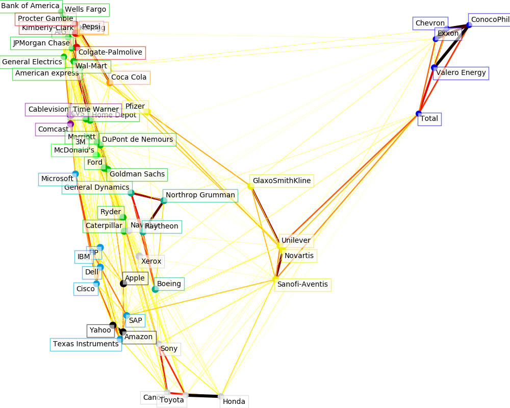
可视化
这三个模型的输出组合在一个2D图中,其中节点表示股票和边界:
聚类标签用于定义节点的颜色。 用稀疏协方差模型表示边缘的强度。 2D嵌入用于在计划中定位节点。
此示例包含大量与可视化相关的代码,因为在这里可视化对于显示图形至关重要。其中一个挑战是定位标签尽量减少重叠。为此,我们使用了一种基于最近邻沿每个轴的方向的启发式方法。
Fetching quote history for 'AAPL'
Fetching quote history for 'AIG'
Fetching quote history for 'AMZN'
Fetching quote history for 'AXP'
Fetching quote history for 'BA'
Fetching quote history for 'BAC'
Fetching quote history for 'CAJ'
Fetching quote history for 'CAT'
Fetching quote history for 'CL'
Fetching quote history for 'CMCSA'
Fetching quote history for 'COP'
Fetching quote history for 'CSCO'
Fetching quote history for 'CVC'
Fetching quote history for 'CVS'
Fetching quote history for 'CVX'
Fetching quote history for 'DD'
Fetching quote history for 'DELL'
Fetching quote history for 'F'
Fetching quote history for 'GD'
Fetching quote history for 'GE'
Fetching quote history for 'GS'
Fetching quote history for 'GSK'
Fetching quote history for 'HD'
Fetching quote history for 'HMC'
Fetching quote history for 'HPQ'
Fetching quote history for 'IBM'
Fetching quote history for 'JPM'
Fetching quote history for 'K'
Fetching quote history for 'KMB'
Fetching quote history for 'KO'
Fetching quote history for 'MAR'
Fetching quote history for 'MCD'
Fetching quote history for 'MMM'
Fetching quote history for 'MSFT'
Fetching quote history for 'NAV'
Fetching quote history for 'NOC'
Fetching quote history for 'NVS'
Fetching quote history for 'PEP'
Fetching quote history for 'PFE'
Fetching quote history for 'PG'
Fetching quote history for 'R'
Fetching quote history for 'RTN'
Fetching quote history for 'SAP'
Fetching quote history for 'SNE'
Fetching quote history for 'SNY'
Fetching quote history for 'TM'
Fetching quote history for 'TOT'
Fetching quote history for 'TWX'
Fetching quote history for 'TXN'
Fetching quote history for 'UN'
Fetching quote history for 'VLO'
Fetching quote history for 'WFC'
Fetching quote history for 'WMT'
Fetching quote history for 'XOM'
Fetching quote history for 'XRX'
Fetching quote history for 'YHOO'
Cluster 1: Apple, Amazon, Yahoo
Cluster 2: Comcast, Cablevision, Time Warner
Cluster 3: ConocoPhillips, Chevron, Total, Valero Energy, Exxon
Cluster 4: Cisco, Dell, HP, IBM, Microsoft, SAP, Texas Instruments
Cluster 5: Boeing, General Dynamics, Northrop Grumman, Raytheon
Cluster 6: AIG, American express, Bank of America, Caterpillar, CVS, DuPont de Nemours, Ford, General Electrics, Goldman Sachs, Home Depot, JPMorgan Chase, Marriott, 3M, Ryder, Wells Fargo, Wal-Mart
Cluster 7: McDonald's
Cluster 8: GlaxoSmithKline, Novartis, Pfizer, Sanofi-Aventis, Unilever
Cluster 9: Kellogg, Coca Cola, Pepsi
Cluster 10: Colgate-Palmolive, Kimberly-Clark, Procter Gamble
Cluster 11: Canon, Honda, Navistar, Sony, Toyota, Xerox
# Author: Gael Varoquaux gael.varoquaux@normalesup.org
# License: BSD 3 clause

import sys

import numpy as np
import matplotlib.pyplot as plt
from matplotlib.collections import LineCollection

import pandas as pd

from sklearn import cluster, covariance, manifold

print(__doc__)


# #############################################################################
# Retrieve the data from Internet

# The data is from 2003 - 2008. This is reasonably calm: (not too long ago so
# that we get high-tech firms, and before the 2008 crash). This kind of
# historical data can be obtained for from APIs like the quandl.com and
# alphavantage.co ones.

symbol_dict = {
    'TOT': 'Total',
    'XOM': 'Exxon',
    'CVX': 'Chevron',
    'COP': 'ConocoPhillips',
    'VLO': 'Valero Energy',
    'MSFT': 'Microsoft',
    'IBM': 'IBM',
    'TWX': 'Time Warner',
    'CMCSA': 'Comcast',
    'CVC': 'Cablevision',
    'YHOO': 'Yahoo',
    'DELL': 'Dell',
    'HPQ': 'HP',
    'AMZN': 'Amazon',
    'TM': 'Toyota',
    'CAJ': 'Canon',
    'SNE': 'Sony',
    'F': 'Ford',
    'HMC': 'Honda',
    'NAV': 'Navistar',
    'NOC': 'Northrop Grumman',
    'BA': 'Boeing',
    'KO': 'Coca Cola',
    'MMM': '3M',
    'MCD': 'McDonald\'s',
    'PEP': 'Pepsi',
    'K': 'Kellogg',
    'UN': 'Unilever',
    'MAR': 'Marriott',
    'PG': 'Procter Gamble',
    'CL': 'Colgate-Palmolive',
    'GE': 'General Electrics',
    'WFC': 'Wells Fargo',
    'JPM': 'JPMorgan Chase',
    'AIG': 'AIG',
    'AXP': 'American express',
    'BAC': 'Bank of America',
    'GS': 'Goldman Sachs',
    'AAPL': 'Apple',
    'SAP': 'SAP',
    'CSCO': 'Cisco',
    'TXN': 'Texas Instruments',
    'XRX': 'Xerox',
    'WMT': 'Wal-Mart',
    'HD': 'Home Depot',
    'GSK': 'GlaxoSmithKline',
    'PFE': 'Pfizer',
    'SNY': 'Sanofi-Aventis',
    'NVS': 'Novartis',
    'KMB': 'Kimberly-Clark',
    'R': 'Ryder',
    'GD': 'General Dynamics',
    'RTN': 'Raytheon',
    'CVS': 'CVS',
    'CAT': 'Caterpillar',
    'DD': 'DuPont de Nemours'}


symbols, names = np.array(sorted(symbol_dict.items())).T

quotes = []

for symbol in symbols:
    print('Fetching quote history for %r' % symbol, file=sys.stderr)
    url = ('https://raw.githubusercontent.com/scikit-learn/examples-data/'
           'master/financial-data/{}.csv')
    quotes.append(pd.read_csv(url.format(symbol)))

close_prices = np.vstack([q['close'] for q in quotes])
open_prices = np.vstack([q['open'] for q in quotes])

# The daily variations of the quotes are what carry most information
variation = close_prices - open_prices


# #############################################################################
# Learn a graphical structure from the correlations
edge_model = covariance.GraphicalLassoCV()

# standardize the time series: using correlations rather than covariance
# is more efficient for structure recovery
X = variation.copy().T
X /= X.std(axis=0)
edge_model.fit(X)

# #############################################################################
# Cluster using affinity propagation

_, labels = cluster.affinity_propagation(edge_model.covariance_,
                                         random_state=0)
n_labels = labels.max()

for i in range(n_labels + 1):
    print('Cluster %i: %s' % ((i + 1), ', '.join(names[labels == i])))

# #############################################################################
# Find a low-dimension embedding for visualization: find the best position of
# the nodes (the stocks) on a 2D plane

# We use a dense eigen_solver to achieve reproducibility (arpack is
# initiated with random vectors that we don't control). In addition, we
# use a large number of neighbors to capture the large-scale structure.
node_position_model = manifold.LocallyLinearEmbedding(
    n_components=2, eigen_solver='dense', n_neighbors=6)

embedding = node_position_model.fit_transform(X.T).T

# #############################################################################
# Visualization
plt.figure(1, facecolor='w', figsize=(10, 8))
plt.clf()
ax = plt.axes([0., 0., 1., 1.])
plt.axis('off')

# Display a graph of the partial correlations
partial_correlations = edge_model.precision_.copy()
d = 1 / np.sqrt(np.diag(partial_correlations))
partial_correlations *= d
partial_correlations *= d[:, np.newaxis]
non_zero = (np.abs(np.triu(partial_correlations, k=1)) > 0.02)

# Plot the nodes using the coordinates of our embedding
plt.scatter(embedding[0], embedding[1], s=100 * d ** 2, c=labels,
            cmap=plt.cm.nipy_spectral)

# Plot the edges
start_idx, end_idx = np.where(non_zero)
# a sequence of (*line0*, *line1*, *line2*), where::
#            linen = (x0, y0), (x1, y1), ... (xm, ym)
segments = [[embedding[:, start], embedding[:, stop]]
            for start, stop in zip(start_idx, end_idx)]
values = np.abs(partial_correlations[non_zero])
lc = LineCollection(segments,
                    zorder=0, cmap=plt.cm.hot_r,
                    norm=plt.Normalize(0, .7 * values.max()))
lc.set_array(values)
lc.set_linewidths(15 * values)
ax.add_collection(lc)

# Add a label to each node. The challenge here is that we want to
# position the labels to avoid overlap with other labels
for index, (name, label, (x, y)) in enumerate(
        zip(names, labels, embedding.T)):

    dx = x - embedding[0]
    dx[index] = 1
    dy = y - embedding[1]
    dy[index] = 1
    this_dx = dx[np.argmin(np.abs(dy))]
    this_dy = dy[np.argmin(np.abs(dx))]
    if this_dx > 0:
        horizontalalignment = 'left'
        x = x + .002
    else:
        horizontalalignment = 'right'
        x = x - .002
    if this_dy > 0:
        verticalalignment = 'bottom'
        y = y + .002
    else:
        verticalalignment = 'top'
        y = y - .002
    plt.text(x, y, name, size=10,
             horizontalalignment=horizontalalignment,
             verticalalignment=verticalalignment,
             bbox=dict(facecolor='w',
                       edgecolor=plt.cm.nipy_spectral(label / float(n_labels)),
                       alpha=.6))

plt.xlim(embedding[0].min() - .15 * embedding[0].ptp(),
         embedding[0].max() + .10 * embedding[0].ptp(),)
plt.ylim(embedding[1].min() - .03 * embedding[1].ptp(),
         embedding[1].max() + .03 * embedding[1].ptp())

plt.show()
脚本的总运行时间:(0分9.212秒)