

单个估计器 vs bagging:偏差-方差分解
此示例说明并比较了单个估计器的期望均方误差与bagging 集成的偏差-方差分解。
在回归中,估计器的期望均方误差可以用偏差、方差和噪声来分解。在回归问题的平均数据集上,偏差项度量了估计器的预测与最优的可能的估计器的预测之间的不同的平均差异, 对问题而言(即Bayes模型)。方差项度量了对于问题而言,当拟合不同的实例LS的时候, 估计器的预测的变化程度。
最后,噪声度量误差的不可约部分,这是由于数据的变异性。
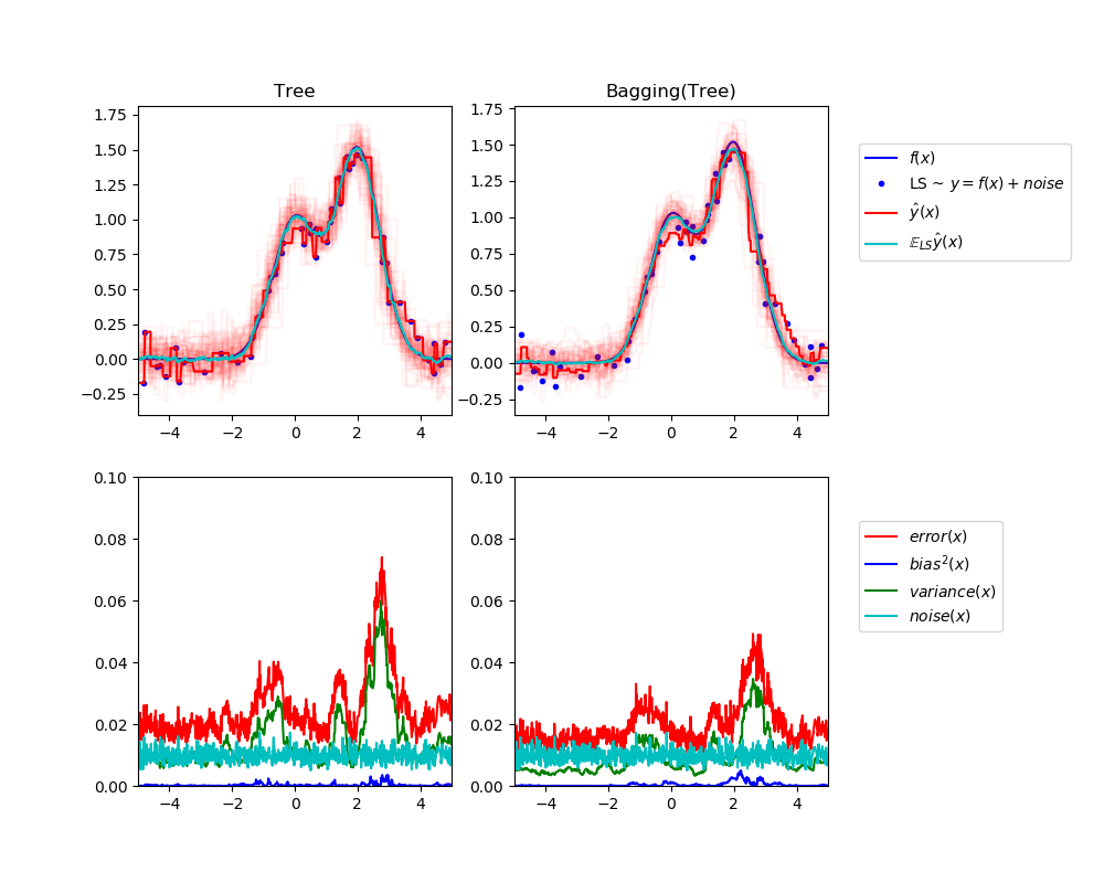
左上角的图说明了一维回归问题, 在玩具的随机数据集LS(蓝点)上训练的单个决策树的预测(以暗红色表示)。它还说明了在其他随机绘制实例LS上训练的其他单个决策树的预测(以淡红色表示)。显而易见地,这里的方差项对应于单个估计器的预测光束的宽度(以亮红色表示)。方差越大,x对训练集中微小变化的预测就越敏感。偏差项对应于估计器(青色)的平均预测值与最佳模型(深蓝色)之间的差异。在这个问题上,我们可以观察到偏差很小(蓝曲线和青色曲线都很接近),而方差很大(红色光束比较宽)。
左下角图描绘了单个决策树的期望均方误差的点态分解。它证实了偏差项(蓝色)是低的,而方差是大的(绿色)。它还说明了误差的噪声部分,如预期的,似乎是恒定的,在0.01左右。
右边的图对应是一样的,但使用的bagging集成的一组决策树。在这两个图中,我们可以观察到偏差项比以前的情况要大。在右上角图中,平均预测值(青色)与最佳模型之间的差异较大(例如,注意x=2附近的偏移量)。在右下角图中,偏置曲线也略高于左下角图。然而,就方差而言,预测束较窄,表明方差较小。事实上,正如右下角的数字所证实的,方差项(绿色)比单个决策树的方差项要低。总的来说,偏差-方差分解不再是相同的。这种折衷更适合于bagging:在数据集的副本上平均几个决策树的结果会略微增加偏差项,但允许更大程度地减少方差,从而导致整体均方误差较低(比较下图中的红色曲线)。脚本输出也证实了这种直觉。bagging的总误差小于单棵决策树的总误差,这种差异确实主要是由于方差的减小所致。
关于偏差-方差分解的更多细节,见[1]中的7.3章节。
参考
1 T. Hastie, R. Tibshirani and J. Friedman, “Elements of Statistical Learning”, Springer, 2009.
Tree: 0.0255 (error) = 0.0003 (bias^2)  + 0.0152 (var) + 0.0098 (noise)
Bagging(Tree): 0.0196 (error) = 0.0004 (bias^2)  + 0.0092 (var) + 0.0098 (noise)
print(__doc__)

# Author: Gilles Louppe <g.louppe@gmail.com>
# License: BSD 3 clause

import numpy as np
import matplotlib.pyplot as plt

from sklearn.ensemble import BaggingRegressor
from sklearn.tree import DecisionTreeRegressor

# Settings
n_repeat = 50       # Number of iterations for computing expectations
n_train = 50        # Size of the training set
n_test = 1000       # Size of the test set
noise = 0.1         # Standard deviation of the noise
np.random.seed(0)

# Change this for exploring the bias-variance decomposition of other
# estimators. This should work well for estimators with high variance (e.g.,
# decision trees or KNN), but poorly for estimators with low variance (e.g.,
# linear models).
estimators = [("Tree", DecisionTreeRegressor()),
              ("Bagging(Tree)", BaggingRegressor(DecisionTreeRegressor()))]

n_estimators = len(estimators)


# Generate data
def f(x):
    x = x.ravel()

    return np.exp(-x ** 2) + 1.5 * np.exp(-(x - 2) ** 2)


def generate(n_samples, noise, n_repeat=1):
    X = np.random.rand(n_samples) * 10 - 5
    X = np.sort(X)

    if n_repeat == 1:
        y = f(X) + np.random.normal(0.0, noise, n_samples)
    else:
        y = np.zeros((n_samples, n_repeat))

        for i in range(n_repeat):
            y[:, i] = f(X) + np.random.normal(0.0, noise, n_samples)

    X = X.reshape((n_samples, 1))

    return X, y


X_train = []
y_train = []

for i in range(n_repeat):
    X, y = generate(n_samples=n_train, noise=noise)
    X_train.append(X)
    y_train.append(y)

X_test, y_test = generate(n_samples=n_test, noise=noise, n_repeat=n_repeat)

plt.figure(figsize=(10, 8))

# Loop over estimators to compare
for n, (name, estimator) in enumerate(estimators):
    # Compute predictions
    y_predict = np.zeros((n_test, n_repeat))

    for i in range(n_repeat):
        estimator.fit(X_train[i], y_train[i])
        y_predict[:, i] = estimator.predict(X_test)

    # Bias^2 + Variance + Noise decomposition of the mean squared error
    y_error = np.zeros(n_test)

    for i in range(n_repeat):
        for j in range(n_repeat):
            y_error += (y_test[:, j] - y_predict[:, i]) ** 2

    y_error /= (n_repeat * n_repeat)

    y_noise = np.var(y_test, axis=1)
    y_bias = (f(X_test) - np.mean(y_predict, axis=1)) ** 2
    y_var = np.var(y_predict, axis=1)

    print("{0}: {1:.4f} (error) = {2:.4f} (bias^2) "
          " + {3:.4f} (var) + {4:.4f} (noise)".format(name,
                                                      np.mean(y_error),
                                                      np.mean(y_bias),
                                                      np.mean(y_var),
                                                      np.mean(y_noise)))

    # Plot figures
    plt.subplot(2, n_estimators, n + 1)
    plt.plot(X_test, f(X_test), "b", label="$f(x)$")
    plt.plot(X_train[0], y_train[0], ".b", label="LS ~ $y = f(x)+noise$")

    for i in range(n_repeat):
        if i == 0:
            plt.plot(X_test, y_predict[:, i], "r", label=r"$\^y(x)$")
        else:
            plt.plot(X_test, y_predict[:, i], "r", alpha=0.05)

    plt.plot(X_test, np.mean(y_predict, axis=1), "c",
             label=r"$\mathbb{E}_{LS} \^y(x)$")

    plt.xlim([-5, 5])
    plt.title(name)

    if n == n_estimators - 1:
        plt.legend(loc=(1.1, .5))

    plt.subplot(2, n_estimators, n_estimators + n + 1)
    plt.plot(X_test, y_error, "r", label="$error(x)$")
    plt.plot(X_test, y_bias, "b", label="$bias^2(x)$"),
    plt.plot(X_test, y_var, "g", label="$variance(x)$"),
    plt.plot(X_test, y_noise, "c", label="$noise(x)$")

    plt.xlim([-5, 5])
    plt.ylim([0, 0.1])

    if n == n_estimators - 1:

        plt.legend(loc=(1.1, .5))

plt.subplots_adjust(right=.75)
plt.show()
脚本的总运行时间:(0分1.587秒)

