

两类的Adaboost
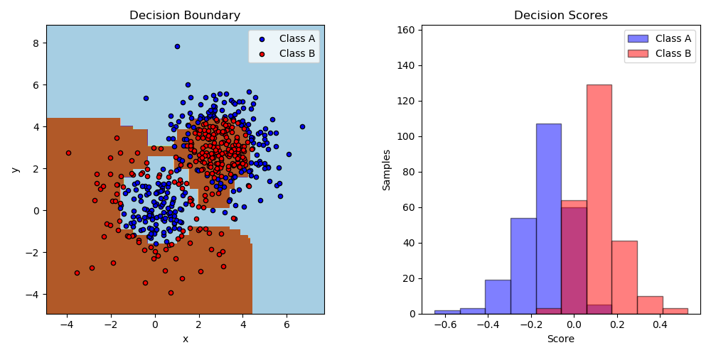
这个例子里面拟合了一个AdaBoosted的决策支柱,使用的数据集是由两个‘高斯分位数’(参看sklearn.datasets.make_gaussian_quantiles)组成的非线性可分的分类数据集, 并绘制决策边界和决策分数。对于A类和B类样本,分别给出了决策分数的分布。每个样本的预测类别标签是由决策分数的符号决定的。决策分数大于0的样本被分类为B,否则被分类为A。决策评分的大小决定了与预测的类标签相似的程度。此外,还可以构造一个包含B类的新数据集,例如,仅选择决策分数高于某个值的样本。
print(__doc__)

# Author: Noel Dawe <noel.dawe@gmail.com>
#
# License: BSD 3 clause

import numpy as np
import matplotlib.pyplot as plt

from sklearn.ensemble import AdaBoostClassifier
from sklearn.tree import DecisionTreeClassifier
from sklearn.datasets import make_gaussian_quantiles


# Construct dataset
X1, y1 = make_gaussian_quantiles(cov=2.,
                                 n_samples=200, n_features=2,
                                 n_classes=2, random_state=1)
X2, y2 = make_gaussian_quantiles(mean=(3, 3), cov=1.5,
                                 n_samples=300, n_features=2,
                                 n_classes=2, random_state=1)
X = np.concatenate((X1, X2))
y = np.concatenate((y1, - y2 + 1))

# Create and fit an AdaBoosted decision tree
bdt = AdaBoostClassifier(DecisionTreeClassifier(max_depth=1),
                         algorithm="SAMME",
                         n_estimators=200)

bdt.fit(X, y)

plot_colors = "br"
plot_step = 0.02
class_names = "AB"

plt.figure(figsize=(10, 5))

# Plot the decision boundaries
plt.subplot(121)
x_min, x_max = X[:, 0].min() - 1, X[:, 0].max() + 1
y_min, y_max = X[:, 1].min() - 1, X[:, 1].max() + 1
xx, yy = np.meshgrid(np.arange(x_min, x_max, plot_step),
                     np.arange(y_min, y_max, plot_step))

Z = bdt.predict(np.c_[xx.ravel(), yy.ravel()])
Z = Z.reshape(xx.shape)
cs = plt.contourf(xx, yy, Z, cmap=plt.cm.Paired)
plt.axis("tight")

# Plot the training points
for i, n, c in zip(range(2), class_names, plot_colors):
    idx = np.where(y == i)
    plt.scatter(X[idx, 0], X[idx, 1],
                c=c, cmap=plt.cm.Paired,
                s=20, edgecolor='k',
                label="Class %s" % n)
plt.xlim(x_min, x_max)
plt.ylim(y_min, y_max)
plt.legend(loc='upper right')
plt.xlabel('x')
plt.ylabel('y')
plt.title('Decision Boundary')

# Plot the two-class decision scores
twoclass_output = bdt.decision_function(X)
plot_range = (twoclass_output.min(), twoclass_output.max())
plt.subplot(122)
for i, n, c in zip(range(2), class_names, plot_colors):
    plt.hist(twoclass_output[y == i],
             bins=10,
             range=plot_range,
             facecolor=c,
             label='Class %s' % n,
             alpha=.5,
             edgecolor='k')
x1, x2, y1, y2 = plt.axis()
plt.axis((x1, x2, y1, y2 * 1.2))
plt.legend(loc='upper right')
plt.ylabel('Samples')
plt.xlabel('Score')
plt.title('Decision Scores')

plt.tight_layout()
plt.subplots_adjust(wspace=0.35)
plt.show()
脚本的总运行时间:(0分3.020秒)

